Summary
Investing with leverage means borrowing money to buy stocks/ETFs/etc. In theory, leverage offers higher expected ending wealth but also higher (systematic) risk and usually even lower median ending wealth. Leverage is not for everyone, even all altruists, but if you have money you want to donate down the road that you can afford to lose without major consequences, then investing it with leverage may be a reasonable choice.
Investing with margin on Interactive Brokers is probably the standard beginner way to achieve long-term leverage. In theory, buying and holding leveraged ETFs could offer an even easier solution (while costing a ~1% expense ratio), but some friends who know more about finance than I do have advised me that daily-rebalanced leveraged ETFs may systematically lose out on their rebalancing trades, such as due to frontrunning.
Before getting carried away with the details of whether and how to use leverage, the more important question is how much of your money, if any, to invest at all compared against donating now. I personally plan to donate most of my future earnings immediately, while saving some money to invest with leverage for donating later.
For further analysis of this topic in the context of effective altruism, see Dickens (2020) and the comments on that post. I don't agree with all of the claims made in that post, but I think it clearly outlines some important issues to think about.
Note added : The default parameters I used in my simulation in this piece were in retrospect too conservative and therefore didn't show leverage performing as well as it probably would in reality. I used a volatility of 22%, but I guess volatilities are usually lower than that (although there are some high spikes), especially when you're diversifying globally. And I used a margin interest rate of 3%, while in fact Interactive Brokers margin interest rates during much of the 2010s decade were I think only a little bit above 1%? Interest rates during the 2010s were extremely low by historical standards, and I was trying to make my calculations more future-proof by choosing an interest rate somewhat closer to the historical baseline. However, it's unclear if and when interest rates will rise again, and if you're investing any time soon, you'd obviously want to do the calculations using the current interest rates rather than my made-up 3% number.
Caveats
This is an advanced topic, so unless you're familiar with the basics of personal finance already, your time is better spent first reading more introductory articles/books.
I'm not a professional investor or economist. This piece relies on the best understanding I've been able to gather as an amateur, and I have only minimal hands-on experience with leveraged investing. There may be errors in my analysis, so I encourage readers to give me feedback. I found several nontrivial bugs in my simulation code over the course of testing it, so it's possible that more bugs remain despite my successful efforts to check the simulation results against theory. Also, my discussion assumes you live in the USA, and many details (especially about taxes) may not extend to other countries.
Contents
- Summary
- Introduction
- Should you invest before donating?
- Possible leverage methods
- IRA to avoid taxes?
- Warnings
- Leverage for retirement?
- Theoretical leverage performance
- What's your altruistic risk tolerance?
- Margin simulations
- Results
- Input parameters for these results:
- How the simulation works
- Results vs. theory
- Validating the results of regular investing
- Validating the results of margin investing
- Prob[margin beats regular]
- Relaxing the simplifying assumptions
- From simple scenario, relax assumption of only earning one initial paycheck
- From that, relax assumption of maintaining leverage equal to broker max
- From that, relax assumption of not tapering off leverage toward end
- From that, relax assumption of no black swans
- From that, relax assumption of no taxes
- From that, relax assumption of no inflation
- From that, relax assumption of no unemployment
- 401k matching beats leverage
- Donor-advised fund vs. leverage
- ESPP plans
- Optimal leverage
- Different margin investing policies
- No emergency savings
- Emergency savings = $1 million
- Don't taper off leverage near end of investing period
- Taper off leverage a lot near end of investing period
- Don't rebalance monthly
- Don't rebalance monthly and don't taper off leverage toward end
- Don't rebalance monthly and pay principal throughout
- Discussion
- Parameter sensitivity analysis
- Assume that Interactive Brokers margin liquidations sell the most tax-advantaged lots first
- Use VIX daily volatilities
- Invest for 5 years instead of 15
- Invest for 30 years instead of 15
- Unemployment lasts a long time
- μ = 0.1
- μ = 0.1 and don't rebalance monthly
- μ = 0.07
- μ = 0.04
- μ = -0.02
- σ = 0.40
- σ = 0, no black swans, no unemployment
- Margin interest rate = 1.5%
- Further simulation features that could be implemented
- Constant-debt investing
- Leveraged ETFs
- Leveraged ETFs vs. margin investing
- Shorting leveraged ETFs?
- Should you have both leveraged and unleveraged investments?
- My plan for using leverage
- A note on refreshing this essay
- Footnotes
Introduction
Many financial commentators advise against leveraging investments due to the higher risk involved. An excellent, simple, graphical tutorial on leverage is "The Danger of Leverage and volatility". I agree it's generally true that most individuals shouldn't leverage non-retirement assets if they plan to use those assets for personal consumption.
But what if you plan to donate the invested assets? You should generally be less risk-averse with funds you plan to donate than with funds you plan to spend on yourself because the marginal altruistic utility of donated dollars usually doesn't decline as sharply as the marginal egoistic utility of dollars for personal consumption.
In the altruistic case, the high-risk / high-expected-value tradeoff that leverage entails is more promising, though the question of whether and how much to use leverage varies from situation to situation. For instance, if a small startup charity is relying on your donations to get off the ground, you probably shouldn't leverage the funds devoted to that purpose unless you can replace any potential investment losses. Basically, only leverage money you can stand to lose.
Should you invest before donating?
This piece is mainly targeted toward altruists who want to donate a few years or decades down the road but are saving their money for now, perhaps because they want to wait to pick out charities or because their desired charities don't yet exist. Some people also think the returns on capital-market investments exceed the returns on direct altruism work. But before jumping into details about whether to invest using leverage, you should first ask: Do I want to invest before donating at all?
There's much discussion regarding the question of whether to donate now or later. For my personal situation, I think the optimal strategy is to donate some amount now toward projects that are either very underfunded or that should be done sooner rather than later. For instance, the Foundational Research Institute is more urgent than a regular charity because its conclusions will help me direct the remainder of my donations. For some other donations, I'd rather wait at least a decade, because I'm continuing to learn a lot, and my opinions will change with new insights.
Possible leverage methods
Following are some methods that are often proposed for leveraging investments. I haven't tried any of them yet firsthand, though I hope to experiment with margin investing soon. Chapter 8 of Lifecycle Investing by Ian Ayres and Barry Nalebuff also surveys these leverage methods.
Margin
Margin investing involves borrowing money from a broker to buy additional stocks/ETFs. By far the best margin rates are offered by Interactive Brokers. However, note that Interactive Brokers requires that you have a minimum account balance of $10K, a minimum liquid net worth of $100K, and experience making at least 100 securities trades on another platform.
Arguments for margin:
- It's more clear that margin investing has the returns you'd expect, because it doesn't rely on market pricing of options and futures.
- Margin buying is sometimes advocated even for normal investors, such as by Manulife Bank of Canada. This increases my confidence that the strategy probably works.
- Unlike options, futures, and the assets traded by managers of leveraged ETFs, if you buy stocks/ETFs on margin, you can hold them indefinitely unless you need to sell to rebalance your portfolio. This means you can potentially hold securities for many years and then donate them when you're ready, thereby never incurring capital-gains tax. In contrast, options and futures typically need to be sold at least once per year, and leveraged ETFs may incur some tax costs through daily rebalancing. Frequent buying and selling also incurs some transactions costs via trading fees and bid-ask spreads.
- In the USA, margin interest can offset net investment income, thereby potentially reducing taxes.
Arguments against margin:
- It requires some work to manually watch your leverage amount, to pay margin interest, and to record all of this on tax returns. The Interactive Brokers platform also has a significant learning curve.
Margin accounts don't allow for high leverage ratios (e.g., 10X or 20X) the way options and futures do. That said, high leverage ratios also require diligent monitoring, since if the price drops even a small amount, you might need to sell many of your assets. For instance, a 5% price drop with 20X leverage destroys your whole account. (This is because if your total assets are $20, $19 of them are debt, and a 5% drop in prices reduces your assets to $19, which can just pay off your debt with nothing left over.) The authors of Lifecycle Investing suggest a maximum of 2X leverage.
Options
Lifecycle Investing recommends buying long call options at about half the current price of the underlying security for ~2X leverage. A Bogleheads thread describes more details.
A friend tells me the following:
About options, you want your effective interest rate to be as close to the risk free rate as possible. To do that, you want as little time value as possible. That means deep in the money call options, although a synthetic stock is reasonable [...].
In other words, the cost of insurance against price drops below the strike price is minimal for deep-in-the-money calls. Alternatively, you could make up for the insurance cost implicit in a call option by selling its corresponding put.
Arguments for options:
- Implied margin interest rates might be competitive for highly liquid options markets, though a friend reports that implied interest rates are unfavorable for thinner markets.
- Unlike with margin investing and futures, you can't lose more money than you invested. The worst case is that you lose everything you put in.
- (Not sure if this is true.) A minor consideration is that because options don't pay dividends, you don't have to pay income tax on dividends in a taxable account. (But this is more than counteracted by needing to pay capital-gains taxes when you sell the options themselves. For example, say you have $100 to invest. You could buy $200 of stocks using 2X margin leverage. If the stocks paid 2% dividends in the year, you'd have to pay taxes on $4 of dividends. In contrast, if you bought $100 of options and they went up, say, 7% by next year, you'd pay taxes on $7 of capital gains. Capital gains if you own stocks directly can be ignored if you continue holding the stocks until you donate them to a tax-qualified charity, whereas you can't hold an option for many years.)
Arguments against options:
- Need to sell every year or so, which means paying capital-gains taxes that you could avoid from buy-and-hold margin investing. As an example, suppose you sell a LEAP every 11 months, and say this gives an annual expected return of 7%. Because your capital gains are short-term, you pay, e.g., 28% tax on the gains. That leaves you with a 5% post-tax return. The situation is less bad if you also have some capital losses to counteract gains.
- It appears that out-of-the-money call options have very bad expected returns, contrary to theoretical predictions that they should have very good expected returns. Paul Christiano seems to suggest that one explanation for this could be that out-of-the-money options are thinly traded. I don't know the answer to the puzzle, but the fact that returns can deviate so sharply from theory at least makes me worried about using options in other contexts. I'd like to learn more about option returns deep in the money (which is the moneyness that Lifecycle Investing encourages), but in the meantime, an ordinary margin account seems safer. Note that leveraged ETFs (discussed more below) also tend to use options (and futures, swaps, etc.) for leverage, and leveraged ETFs track their desired targets very closely on a daily basis.
- A friend tells me: "I've been disappointed with options as a source of leverage. Compared to margin loans, there aren't many securities with options. And of securities with options, many of those options are illiquid and basically can't be traded. Of those options that can be traded, the effective interest rate is considerably higher than [Interactive Brokers]'s highest margin rate." SPY may have low-ish implied interest rates, but as is discussed later, there are reasonable concerns about levering the US stock market in particular as of ~2015.
Index futures
Buying futures on, say, the S&P 500 index can multiply your market exposure possibly 10X or 20X. I haven't explored this option enough to comment much on it.
Arguments for futures:
- If you want extremely high leverage, index futures are probably the way to go. (However, only the most risk-neutral altruists might want such high degrees of leverage.)
Arguments against futures:
- Need to sell every ~3 months or so, which means paying capital-gains taxes that you could avoid if you used buy-and-hold investing.
Leveraged ETFs
Arguments for leveraged ETFs:
- By far the easiest way to get leverage, since you can buy them in a normal brokerage account without setting up margin or options/futures trading. If you buy and hold, you can also just leave them alone until you want to dispose of them.
- Unlike with margin investing and futures, you can't lose more money than you invested. The worst case is that you lose everything you put in.
- (Not sure if this is true for all leveraged ETFs.) Since leveraged ETFs use non-dividend-paying derivatives to achieve leverage, they tend not to have distributions, which is good if you're in a taxable account.a However, this point may be small compared with the higher taxes that leveraged ETFs may pay on average compared with regular ETFs.
Arguments against leveraged ETFs:
- The expense ratios may be ~1% for a service that you could mostly replicate on your own with a margin account.
- Due to turnover of the assets in the fund, taxes may be greater than with buy-and-hold margin investing, and capital gains may often be treated as short-term regardless of how long you hold the fund. According to one page: "Capital gains distributions from leveraged ETFs became an issue in 2008 when Rydex reported distributions of as much as 70% of fund assets. [That is, if the gain was $X, and if your tax bracket was 28%, you would have paid $X * 70% * 28%, or about $X * 20%.] In 2009, Direxion reported moderate capital gains on some of its funds while ProShares reported zero capital gains distributions." Another article quotes Andy O'Rourke: "Both ProShares and Rydex paid zero capital gains on all of the leveraged ETFs. Direxion Shares ETFs also paid capital gains on only 11 of their funds, and no amount greater than 15% of assets." Taxes on distributions from leveraged ETFs are less of an issue for short-term traders, but most of us are not (and should not try to be) short-term traders. Moreover, if you're investing prior to donating to a 501(c)(3) charity, then you never pay capital-gains taxes if you buy and hold, so any premature distributions or capital-gains taxes are bad.
- I assume (?) that frequent buying and selling also means transactions costs, bid/ask spreads, etc.
Home mortgage
A home mortgage is one of the most common forms of leveraged investing (with another being college loans).
Arguments for home mortgages:
- Popular and have common-sense approval.
- Mortgage interest is deductible. Moreover, whereas margin interest is only deductible to offset net investment income, mortgage interest doesn't have the same restriction, so it's deductible even if you have net capital losses. (This is just my impression from cursory reading. Readers, please correct me if it's wrong.) That said, if you don't have other itemized deductions, you might take the standard deduction, in which case there's no benefit to mortgage interest being deductible.
Arguments against home mortgages:
- Mortgage interest rates are higher than margin rates from Interactive Brokers.
Whether to get a home mortgage depends crucially on whether you want to buy a house in general. There's much discussion on that question, and following are a few considerations:
Arguments for buying a house/condo:
- Exclusion from $250K ($500K if married) of capital gains when you sell a house.
- You avoid paying taxes on "rent" to yourself, whereas a landlord pays taxes on rent from a tenant. For example, suppose a living space is worth $1000/month intrinsically. If you own it, you're "paying" yourself $1000/month of rent tax-free. If you instead rent it, since you want to get back $1000/month after taxes (assume a 28% tax rate), you have to charge your tenant $1389/month. Hence, the renter pays more. (Thanks to a friend for this point.)
Arguments against buying a house/condo:
- Buying and selling are a lot of hassle if you move frequently and incur big transaction costs.
- Have to take care of property taxes, repairs, and home improvements yourself. Depending on the neighborhood, you might be required to maintain your lawn.
- Real estate is plausibly a worse investment than stocks because people buy real estate partly as a consumption good, i.e., houses have positive "convenience yield". And historically, houses have probably underperformed stocks, though the difference in performance is much smaller when one considers savings from not paying rent. The Case–Shiller home-price index has increased only ~0.7% per year in real terms since 1940(?).
IRA to avoid taxes?
The tax disadvantages of options and futures can be avoided if you're trading in an IRA. However, note that if you can't get a tax deduction for a traditional IRA, then a non-deductible traditional IRA is a bad deal because you pay income-tax rates both before adding money and when withdrawing it, while investing in a regular brokerage account involves paying income tax on the way in but only long-term capital-gains rates on the way out, assuming you buy and hold until retirement.
If you're ineligible for deductible IRAs because your income is too high, you can still get a backdoor Roth IRA, but it's not clear that this will continue to work forever, and managing one requires nontrivial effort for only ~$5500 of contributions per year. Assuming you save well over ~$5500 per year, you'd still need another leverage method for your other investments.
Another risk with margin investing in IRAs is that if you get a margin call and deposit more funds into the account, you might exceed the IRS limits for the maximum amount you can add to the account per year. The Interactive Brokers Margin Disclosure says: "Deposits to the account in excess of [IRS] limits may cause adverse tax consequences, including but not limited to, forfeiture of the tax-advantaged status of the IRA account and/or penalties." That said, this may not be a problem if you always pay margin calls by selling equity rather than depositing more funds.
Warnings
General
Except for buying leveraged ETFs (which is easy), investing with leverage requires some sophistication. Try it out with small amounts of money at first, until you learn the mechanics and tax implications.
About Interactive Brokers
The Interactive Brokers (IB) Customer Agreement warns that IB may liquidate positions if margin exceeds limits without issuing a margin call, i.e., without giving you a chance to add more money. IB reserves the right to liquidate whichever securities they want without telling you. This seems bad because IB might(?) liquidate short-term rather than long-term assets, and capital gains rather than capital losses, thereby increasing the capital-gains taxes you'll pay. To avoid this, I would probably voluntarily maintain a margin amount less than the limit so that I'm the one who manually does rebalancing when necessary.
IB's Customer Agreement also says: "Customer acknowledges Customer's responsibility for knowing the terms of any securities, options, warrants or other products in Customer's account, including upcoming corporate actions (e.g., tender offers, reorganizations, stock splits, etc.). IB has no obligation to notify Customer of deadlines or required actions or dates of meetings, nor is IB obligated to take any action without specific written instructions sent by Customer to IB electronically through the IB website." In fact, IB does provide notifications of corporate actions, so I think this statement from the Customer Agreement was mainly CYA, though it's possible that IB may sometimes fail to report certain notifications or updates. In any case, this warning is something to keep in mind if you own individual stocks. (It's probably less important if you only own index/sector ETFs, since I don't think they have corporate actions.) Responding to corporate actions is important. I own individual stocks in my non-IB brokerage account, and I would guess that ~1-3% of them per year have issued tender offers, which require shareholders to either accept the offer or sell the security before it becomes worthless. If you miss the deadline, you just lost the value of the security.
If you already have assets with another broker, you should use ACATS to transfer your securities to Interactive Brokers. You shouldn't sell your securities and then wire the money, because this incurs capital-gains tax! Select only a "Partial" transfer unless you want to move your whole brokerage account. Doing only a partial transfer might save on ACAT fees by your old broker. If you have shares purchased using ESPP, you may need a special form for transferring, so call your broker about that. Since Interactive Brokers says in the quote from the previous paragraph that they may not report corporate actions, I didn't transfer big amounts of small/mid-cap stocks to Interactive Brokers in case Interactive Brokers's reporting of tender offers/etc. is inferior to that of my existing broker, but I hope to learn more about this over time.
IB says they're not liable if your account is hacked if you're not using their secure login. I don't know how this compares with other brokerages, but my guess is that some more consumer-friendly brokerages might be more willing to reimburse money lost due to someone else breaking in to your account. IB does use a special security device to reduce the risk of someone breaking in to your account.
One minor inconvenience that I had when using IB was with gifting my securities to my donor-advised fund. I can gift shares from my non-IB brokerage account to my donor-advised fund fully electronically, because I have a donor-advised fund that's directly connected to my non-IB broker. In contrast, gifting from IB required me to print out a form and physically mail it to my donor-advised fund. Actually, when I tried to transfer shares from IB to my donor-advised fund via a physical letter, IB refused, since they don't handle paper forms. So what I did instead was ACAT the shares from IB to my non-IB brokerage account and then donate from the non-IB brokerage account to my donor-advised fund. ACATS involves an in-kind transfer and so doesn't incur tax.
Invest in foreign ETFs?
Many commentators believe that the US stock market is overpriced as of ~2015. This is suggested by most fundamental-valuation metrics. As a result, it may be best to buy mostly global equity ETFs. Even if you (like me) have strong efficient-market intuitions, it at least shouldn't hurt to buy global ETFs (except for slightly higher expense ratios and bid/ask spreads) in order to reduce exposure to the possible US stock-market bubble as of ~2015.
Social impact of leverage
Using leverage to increase the amount you can donate to charity is very likely a net positive socially. That said, it's worth thinking about the direct social impact of leverage. Usually people say that leveraged investing increases financial instability by amplifying both positive and negative returns. When the market declines, people using leverage have too much debt and so need to sell some of their positions to restore their target leverage ratios, which pushes prices down further.
Margin investing slightly increases demand for loans, pushing interest rates slightly higher. I would also guess that when more money is invested in stocks, the willingness of companies to IPO increases slightly, since companies can expect higher prices for their initial shares, but I haven't read this anywhere, so it could be completely wrong. These seem like small effects, and it's not obvious if they're good or bad anyway.
I would conjecture that more people investing in stocks pushes down long-run (if not short-run) stock-market returns because the fundamental value of the companies being invested in is fixed. If so, then gains from margin investing are zero-sum in the sense that they come at the expense of lower returns by other investors? However, since most investors would spend the money on themselves (and most people who can afford to invest in the stock market are reasonably well off to begin with), this doesn't seem like a huge altruistic downside.
Leverage for retirement?
In addition to relatively risk-neutral altruists, leverage might also appeal to many ordinary investors when it comes to retirement. Lifecycle Investing makes the case that most young people should leverage their investments. Here's a summary of the argument: "Why Young People Should Buy Stocks on Margin". See also "Early Retirement Using Leveraged Investments". I'm not focusing on retirement in this piece, but that is another plausible reason to be interested in leverage.
The simulations I present later in this essay aren't targeted toward retirement, because the hypothetical investors in those simulations maintain constant leverage throughout the investing period, whereas Lifecycle Investing advocates reducing leverage over time to maintain a constant allocation between stocks and bonds when one's future earnings are considered a bond.
Personal retirement thoughts
Personally I'm not that interested in using leverage for retirement because 401k matching is better than leverage, and I expect that matched 401k savings would go a decent way toward supporting me in retirement. In particular, make the following assumptions:
- My employer matches 50% of 401k contributions up to $6K/year. So I would contribute $6K and my employer would contribute $3K for a total of $9K/year.
- These contributions continue for 35 years, and the matching-contributions limit keeps pace with a 3% annual inflation rate.
- 401k investments return a constant 5% nominal return per year.
- Suppose that if I retired now, I'd need $20K/year during retirement. (That's higher than my current costs of living, but maybe I'd have more medical expenses and such.)
- In retirement I'd pay a constant 15% income-tax rate on 401k withdrawals.
This spreadsheet suggests that these 401k contributions would last for ~22 years of retirement.
So maybe these contributions alone wouldn't keep me afloat during retirement, but I could make up for this in various ways:
- Contribute a bit more to my 401k
- Earn some income during retirement, perhaps by continuing to produce writings that others find valuable
- Move to a place with extremely low costs of living
- Go broke and rely on poverty assistance.
Social Security might also help, but I'm not counting on it being around.
In any event, I expect major changes in the world in the coming decades, so these calculations probably ignore substantial factors that will transform the retirement landscape.
Theoretical leverage performance
You might think that because leverage involves holding twice as much equity as regular investing that (ignoring loan interest), the performance of a 2X leveraged position would just be 2 times the performance of regular equity investing, with double the possible gains and double the possible losses, but with the distribution having the same general shape.
This is not how leverage actually performs. Volatility distorts the distribution of outcomes. As a result, 2X leverage usually does worse than twice the underlying asset, and often it does worse than the underlying asset itself. For example, the US SEC issued an alert containing the following anecdote: "Between December 1, 2008, and April 30, 2009, a particular index gained 2 percent. However, a leveraged ETF seeking to deliver twice that index's daily return fell by 6 percent [...]."
So why would anyone use leverage? Because it offers small probabilities of huge gains. Higher and higher leverage amounts become like lottery tickets in a lottery where the expected value is actually better than fair, as will be discussed below.
Simple example
Let's start with a simple case. Something like this is commonly used when discussing leveraged ETFs.
Regular investing
Suppose you have $100 in an index ETF. Imagine there are only two possible returns for the ETF in a given period: up 10% or down 10%. Each has equal probability. Let Ri be a random variable for the return of the ETF in period i. Ri is either .1 or -.1.
There are four possible outcomes, each equally likely:
- $100(1+.1)(1+.1) = $121
- $100(1-.1)(1+.1) = $99
- $100(1+.1)(1-.1) = $99
- $100(1-.1)(1-.1) = $81
Your expected ending wealth is ($121 + $99 + $99 + $81)/4 = $100, just like you'd expect naively. But your median ending wealth is $99. In other words, even regular stock-market investing contains a bias toward losing some money in terms of the median (not mean) outcome. The reason we don't usually notice this is that the stock-market has a general upward trend, which hides this small drag from volatility.
We can approximate the effect of drag as follows. Note that E[Ri] = 0 and Var[Ri] = E[Ri2] - E[Ri]2 = E[Ri2] - 0 = E[.01] = .01. The median outcome was $1 lower than the mean, i.e., was $100 * Var[Ri] lower.
Leveraged investing
The reason the SEC and others warn about leverage is just that it amplifies this volatility drag. To see this, note that a leveraged version of the above ETF would have possible returns of +20% and -20%, giving these four possible outcomes:
- $100(1+.2)(1+.2) = $144
- $100(1-.2)(1+.2) = $96
- $100(1+.2)(1-.2) = $96
- $100(1-.2)(1-.2) = $64
Your expected ending wealth is ($144 + $96 + $96 + $64)/4 = $100, just like before. But the median ending wealth is now $96, and the worst case is much worse. This is typical of leverage: it makes many of the outcomes worse but some of the outcomes vastly better.
Now Var[Ri] = E[Ri2] - E[Ri]2 = E[Ri2] - 0 = E[.04] = .04. The median outcome was $4 lower than the mean, i.e., was $100 * Var[Ri] lower. 2X leverage means 4X variance, so the drag is actually quadratic in the leverage amount.
Geometric Brownian motion model
Regular investing
The most common model of stock-market evolution is geometric Brownian motion. Let St be the price of a stock or ETF at year t. The geometric Brownian motion stochastic differential equation (SDE) is
dSt/St = μ dt + σ dWt,
where μ is the expected annual return, σ is the annual volatility, and Wt is a Weiner process with mean 0 and variance t. That is, if Z is a standard-normal random variable, then dWt = Z√dt.
Solving this SDE tells us that
St = S0 exp(μt - σ2t/2 + σWt). (call this the "regular St equation")
St/S0 has a lognormal distribution with location parameter μt - σ2t/2 and scale parameter σ√t.
The median of a lognormal distribution is exp(location_parameter). Thus
median(St) = S0 exp(μt - σ2t/2) (call this the "regular median equation")
because S0 is constant and so doesn't affect the sorted ranking of St values. We can see the same volatility drag discussed before, in the ‑σ2t/2. See here for more discussion of this "convexity correction" term.
The mean of a lognormal distribution is exp(location_parameter + scale_parameter2/2). Hence
mean(St) = S0 exp(μt), (call this the "regular mean equation")
since the constant S0 can come out of the mean() operator. This equation is confirmed by Wikipedia. We see that volatility doesn't drag down the mean; it just skews the distribution such that most of the outcomes (including the median) are lower.
Leveraged investing
Let Vt denote the net wealth of a leveraged portfolio at year t. (Vt is just like St but for leveraged investing.) Domian et al. (2003) show (p. 5, eqn. 13) that for a c-times leveraged portfolio (e.g., c = 2 means 2X leverage) and borrowing interest rate r, the applicable SDE is
dVt/Vt = (r + (μ-r)c) dt + c σ dWt.
This makes sense because the infinitesimal expected return should be cμ dt, the infinitesimal standard deviation should be cσ √dt, and the infinitesimal borrowing cost should be (c-1)r dt (since only c-1 of the purchased units are borrowed).
Domian et al. (2003) solve this equation (p. 5, eqn. 14) in the same way we solved the regular St equation. The result is
Vt = V0 exp{ (r + (μ-r)c) t - c2σ2t/2 + cσWt }. (call this the "leveraged Vt equation")
Vt/V0 is lognormal with location parameter (r + (μ-r)c) t - c2σ2t/2 and scale parameter cσ√t.
In analogy with before, we have
median(Vt) = V0 exp{location_parameter} = V0 exp{(r + (μ-r)c) t - c2σ2t/2}. (call this the "leveraged median equation")
We can see that the volatility drag is quadratic in the leverage amount (c2).
Likewise:
mean(Vt) = V0 exp(location_parameter + scale_parameter2/2) = V0 exp{(r + (μ-r)c) t - c2σ2t/2 + c2σ2t/2} = V0 exp{(r + (μ-r)c) t}. (call this the "leveraged mean equation")
This result can also be written as V0 exp{[μc-r(c-1)] t}. This is exactly what we would have thought naively: The performance of leveraged investing is c times the underlying asset performance, minus (c-1) times loan interest (since we only take out a loan for c-1 of the total investment amount).
Comparison between regular and leveraged
Consider equal starting investments of $K between a regular (c = 1) and leveraged (c > 1) portfolio: S0 = V0 = K. Suppose μ > r, as is usually the case.
Using the median equations just derived:
= exp{(r + (μ-r)c) t - c2σ2t/2 - μt + σ2t/2 }
= exp{rt + μct - rct + (1 - c2)σ2t/2 - μt }
= exp{ μ(c-1)t - r(c-1)t + (1 - c2)σ2t/2 }
= exp{ (μ-r)(c-1)t + (1 - c2)σ2t/2 }.
The exact appearance of this curve depends on the input parameters. Here's what it looks like with one reasonable set of parameters (including μ = 0.054) and here's with a more optimistic μ=0.09. Most of the time, the curve is less than 1, i.e., using leverage implies a lower median return. Presumably this is a main reason why the SEC warns against leveraged ETFs: They typically do underperform regular ETFs.
However, the story is different when it comes to mean returns. Using the mean equations just derived:
mean(Vt) / mean(St) = [K exp{(r + (μ-r)c) t}] / [K exp(μt)] = exp{(r + (μ-r)c) t - μt)} = exp{rt + μct - rct - μt)} = exp{(μ-r)(c-1)t}.
Since μ-r > 0 and c-1 > 0, this ratio is greater than 1 and increases with t. Here's one sample calculation of this ratio with particular parameter choices:
mean(Vt) / mean(St) = exp{(μ-r)(c-1)t} = exp{(0.054-0.03)(2.0-1) * 15} = 1.43. (call this the "mean(margin)/mean(regular) equation")
For instance, if you can make an expected $100K with normal investments, you'd make (in expectation, not median) $143K with 2.0X leverage.
So (at least in this simplified theoretical model), leverage does indeed offer higher expected ending wealth than non-leveraged investing.
We can prove that leverage has higher expected returns even more simply and generally. Assume that some investment's daily returns Ri are independent and identically distributed with some mean E[R]. The total wealth multiplier after N days is
For independent random variables, the expected value of a product is the product of expected values, so the expected wealth multiplier after N days is
= E[(1+R1)] E[(1+R2)] ... E[(1+RN)]
= (1+E[R]) (1+E[R]) ... (1+E[R])
= (1+E[R])N.
In other words, we maximize expected wealth after N days by maximizing the expected daily return E[R]. Since leverage increases E[R], leverage has higher expected value. Q.E.D.
The catch, of course, is that most investors—even most altruists—shouldn't be risk-neutral with respect to wealth. The next section discusses what levels of risk aversion might be reasonable when it comes to wealth that will be donated.
Also note that this continuous-time model doesn't allow margin accounts to go bankrupt. Because a continuous-time margin account maintains constant leverage, if its assets fall, it rebalances immediately by selling some securities. In the real world, margin accounts can go bankrupt. This could, with low probability, even happen if the account rebalances daily. For instance, a 5X-leveraged margin account that rebalanced once per day might have been wiped out by 1987's Black Monday. By not allowing for bankruptcy (and by ignoring black swans in general), continuous-time equations like those above may slightly overstate the expected value of leverage. In the extreme case, taking t = ∞, a margin investor who doesn't rebalance continuously would go bankrupt with probability 1 (since eventually there would be a huge, near-instantaneous market downturn that destroys the account), while the leveraged mean equation concludes that the margin investor ends up with infinite expected wealth.
What's your altruistic risk tolerance?
Suppose you're donating to support some overall cause, such as safety of artificial general intelligence. Typically a cause has diminishing marginal value with additional dollars. This is for various reasons, such as that the best people are employed first and for the lowest wages, and that lowest-hanging fruit for solving the problem tend to be plucked first.
Within a given cause, some projects may have more value for you than others. For instance, maybe you like one charity a lot more than other charities for the same cause. In that case, maybe looking at just that charity's funding is the right unit of abstraction. But that individual charity will also usually show diminishing marginal value with funding.
Say we've picked some level of abstraction (a cause, a charity, etc.) that we want to fund. It seems plausible that the good g that's accomplished by a given number of dollars d given to that cause/charity is dγ for some γ in the interval (0,1]. γ = 1 corresponds to no diminishing marginal good, but this seems rare. More plausible values of γ might be 0.9 or 0.75 or 0.5.
You are one individual planning to donate to the cause/charity. Let your donation amount be m (short for "myself"). Let the donation amount of all the other donors be o (short for "others"). Then the total good done is g(m+o) = (m+o)γ.
g(d) defines the cause or charity's utility function with respect to total donated dollars. But it's also helpful to define your individual altruistic utility function with respect to dollars you personally donate. Below, I refer to this as utility(wealth), and I approximate it by (wealth)α for some α. It's easy to get this confused with the charity's utility function of dγ for some γ. Just remember that if you see a γ, it reflects the utility function of the charity, while α refers to your personal altruistic utility function with respect to how much money you can personally donate.
Case 1: You are the charity's main donor
If m ≫ o, then g(m+o) is roughly mγ. In such a case, the good you accomplish is roughly your wealth raised to the γ, so for investment decisions, you should maximize expected utility, with utility(wealth) = (wealth)γ. That is, α = γ.
Suppose that m ≪ o, and the returns you earn on your investments aren't appreciably correlated with how much others donate. In this case, the marginal contribution of your donation, m, is
As an example, suppose o = 107 and m ranges between 0 and 106. Basically regardless of γ, utility(wealth) is almost linear in wealth, i.e., α ≈ 1. For instance, here's the curve for γ=0.5.
This is consistent with the naive intuition that if an organization is big, then small amounts of additional donations should have roughly linear impact, since the marginal utility of donations shouldn't level off that much. In particular, if g(d) = dγ, the derivative at o (i.e., you donate nothing) is g'(o) = γ oγ-1, while the derivative at m+o (i.e., you do donate m) is g'(m+o) = γ (m+o)γ-1. The ratio is
o/(m+o) is close to 1 for o ≫ m, and 1-γ is some exponent like 0.1 or 0.5. Taking a fractional exponent of a number slightly less than 1 just makes the result even closer to 1. Hence, the ratio of derivatives is nearly 1, showing that marginal utility doesn't decline that much regardless of how much you donate as long as your donations are small relative to the total.
This scenario makes leverage look promising because for a linear utility function, maximizing expected utility means maximizing expected wealth.
One example of a high-risk situation where your returns aren't highly correlated with those of other donors is entrepreneurship. Carl Shulman suggests that altruistic donors should be more risk-neutral than egoistic spenders.
In most domains besides entrepreneurship, non-systematic risk can be diversified away, so the only risk is systematic risk (called "beta"). The risk from leverage is mainly systematic risk, since the leveraged portfolio aims for a multiple of the underlying asset. Systematic risk is likely to be correlated with others' donations, so we now turn to focusing on that case.
Note: This section is weird, and I'm not at all sure I'm thinking about it correctly. So what I say here may be wrong.
This section expands upon this discussion and takes inspiration from "Risk aversion and investment (for altruists)" by Paul Christiano.
Let St be the normalized value of some underlying market index, like a global equity index fund. By "normalized" I mean that, for instance, it's relative to S0 = $1. You pursue some investment strategy, possibly including leverage, based on St, so your final wealth is a function m(St) of St. Likewise, at least some other donors have exposure to St, so their donations are also a function o(St) of St. For example, suppose that half of other donors have assets uncorrelated with equities, and the other half have everything they plan to donate in the equity index fund or equivalent portfolios. Then o(St) = N * (ξt/2 + St/2), where N is some scaling factor, ξt/2 is the normalized performance of the non-equity assets (which we can ignore as not depending on St), and St/2 is from the equity assets whose donated value is proportional to the index performance.
The value that you contribute by your donation is the difference in good done by the cause/charity with your donations vs. without them:
utility(your wealth) = utility(m(St)) = g(m(St) + o(St)) - g(o(St)) = (m(St) + o(St))γ - o(St)γ.
Our goal in the remainder of this section is to approximate the above equation in the simpler form utility(m(St)) ∝ (m(St))α for some appropriate α, so that we can later evaluate your utility of investment wealth more compactly as just (wealth)α for some α. I wrote "∝" rather than "=" because scalar constants multiplied by a utility function won't affect decisions, since what maximizes expected utility also maximizes expected (k * utility) for any positive constant k.
Suppose o(St) = N Stη for some constant N and some η in the interval [0,∞). This reflects the idea that people give more when the stock market is doing well. If η=1, this means that people's total donations are a constant fraction of their accumulated stock-market assets. (In practice, η could be higher or lower.) Then
utility(m(St)) = (m(St) + N Stη)γ - (N Stη)γ. (call this "utility equation 1")
Say you're following a c-times leveraged strategy, so that m(St) = M Vt, where M is some constant, and Vt is the performance of the leveraged investment, normalized to the same scale as St, e.g., normalized such that V0 = $1. Combining the regular St equation and the leveraged Vt equation and assuming that V0 = S0 = 1:
= exp{ rt + μct - rct - c2σ2t/2 + cσWt - μtc + σ2tc/2 - σcWt }
= exp{ rt - rct - c2σ2t/2 + σ2tc/2 }
= exp{ (1-c)rt + (c-c2)σ2t/2 },
which is a constant (independent of St).b Denote it by q. So
m(St) = M Vt = M q Stc.
Inversely:
[m(St)/(Mq)]1/c = St.
Substituting back into utility equation 1:
utility(m(St)) = (m(St) + N [m(St)/(Mq)]η/c)γ - {N [m(St)/(Mq)]η/c}γ. (call this "utility equation 2")
Finally we have utility purely as a function of your own donation amount that factors in its correlation with others' donations. Now let's see what shape the function has given some plausible parameter values.
Take M = 105, meaning the absolute amount you donate is $100,000 times Vt/V0. Suppose N = 107, which means the scale of others' donations is about 100 times yours. Assume η=1 for simplicity.
Simple scenario: c=1
Suppose you don't leverage investments (c=1). Then q=1. Utility equation 2 becomes
utility(m(St)) = (m(St) + N m(St)/M)γ - (N m(St)/M)γ.
N/M = 100, i.e., total funding for the cause/charity is roughly 100 times your donations. So
= (101 m(St))γ - (100 m(St))γ
= 101γ m(St)γ - 100γ m(St)γ
= (101γ - 100γ) m(St)γ.
For a given γ, the first factor is constant. Hence, the value of your donation scales as utility(wealth) ∝ (wealth)γ—just like it did when we assumed you were the only major donor! This is because, when all donors are perfectly correlated according to market performance, it's as though there's only one big donor (who donates 101 m(St)), and his/her donations have value (wealth)γ.
Scenario: c=2
Let's calculate q with the following parameter choices:
= exp{ (1-2) * 0.03 * 15 + (2-22) * 0.222 * 15/2 }
= 0.3.
Then utility equation 2 becomes
= (m(St) + 107 [m(St)/(30000)]1/2)γ - {107 [m(St)/(30000)]1/2}γ
= (m(St) + 107 √m(St)/173.2)γ - (107 √m(St)/173.2)γ
= (m(St) + 57737 √m(St))γ - (57737 √m(St))γ.
Even for γ = 0.5, say, this curve is relatively linear in m(St), and for γ closer to 1, it's almost perfectly straight.
Scenario: c=3
= exp{ (1-3) * 0.03 * 15 + (3-32) * 0.222 * 15/2 }
= 0.046.
Then utility equation 2 becomes
= (m(St) + 107 [m(St)/(4600)]1/3)γ - {107 [m(St)/(4600)]1/3}γ
= (m(St) + 107 m(St)1/3/16.6)γ - (107 m(St)1/3/16.6)γ
= (m(St) + 602400 m(St)1/3)γ - (602400 m(St)1/3)γ.
Even for γ = 0.5, say, this curve is relatively linear in m(St), and for γ closer to 1, it's almost perfectly straight.
Take-home lessons
- If you're a small donor relative to the total, and if the donations of others aren't significantly correlated with your investment performance, then you should be roughly risk-neutral with your investments, which implies a strong prima facie case for leverage.
- On the other hand, if you're one of the few donors to the cause/charity, or if your investment returns are highly correlated with others' donations and you don't use leverage, then the shape of your utility function for ending wealth will be utility(wealth) ∝ (wealth)γ, where γ reflects the charity's degree of diminishing returns to total financial resources.
- When you use leverage, the utility added by a certain amount of investment return becomes closer to linear in ending wealth (i.e., you become closer to risk-neutral again). I'm not very confident in this conclusion because it's counterintuitive and might be wrong.
In the remainder of this piece, I assume that utility(wealth) = (wealth)α for some fixed value α regardless of leverage, but it's important to note that this assumption is actually not true when there are other donors whose returns are correlated with yours. In this situation, if you use leverage, the correct personal α to use is higher than (and implies a utility function more linear than) the γ value for the cause/charity. Because α increases with leverage, assuming a constant α actually understates the case for leverage. If the cause or charity is tiny and your donations account for most of the funding, then of course a constant α = γ value is indeed appropriate.
In the results below, I present both average wealth (corresponding to α=1) and average √wealth (corresponding to α=0.5). Probably the correct α to use lies somewhere in between these extremes.
Finally, keep in mind that stability of donations might be valuable even apart from diminishing marginal value of additional wealth, since it allows recipient charities to better plan, experience less budget-induced turnover of staff and projects, etc. The analysis of how this affects α might be similar as above:
- If you're the main donor, it argues against variance.
- If you're a small part of all donations and not correlated with others, variance doesn't matter as much because blips up and down can be smoothed out by the recipient organizations to some extent.
- If you're correlated with other donors, then variance again becomes problematic because the organization might lose lots of donations all at once.
That said, if the organization isn't counting on your donations, then these stability arguments become less pressing. If you make a single, big, unexpected donation, the charity can smooth it out over time. If you donate regularly, then variability in how much you donate per period is bad, but if you're drawing down a given accumulation of savings, you can artificially keep donations constant by donating a fixed amount per year regardless of investment performance.
Donating to causes with different γ's
Some of the charities I plan to give toward have relatively low γ's. For instance, the γ of the Foundational Research Institute might be 0.5 or so. Currently I'm one of the main donors, so my personal α is also close to 0.5.
In contrast, the Humane Slaughter Association probably has a cause-wide γ closer to 0.8 or something, since the cause of humane slaughter scales pretty well with additional funding, at least at this stage when many major improvements are still needed. Moreover, the organization already gets ~$500K/year in donations, so an additional donation m between $0 and ~$100K would have roughly linear value with respect to m.
If you're splitting donations among causes like these, I suppose you could use leverage for those savings that you plan to give to organizations where the value of your donation is roughly linear and avoid it for those savings earmarked toward the more risk-averse charities. I don't know if there's a way to merge assets into a single pool with a mix of risk in between the two extremes. Splitting between some leveraged and some regular investments seems clear conceptually and easy to implement.
What about other donations you'll make later?
Modeling utility(wealth) = (wealth)α for only wealth earned over a only part of your life (say, a 15-year period) has a flaw: You'll probably donate more than this later on. Plus, maybe you have other savings not invested on margin that you'll donate as well. In this case, the total amount of your wealth is your current margin investments plus other amounts. In general, this should have the effect of implying that your current donations are actually farther along the utility(lifetime-donated wealth) curve than they seem and hence that marginal utility diminishes less sharply than you might think.c A hacky correction for this observation is to increase α relative to a naive estimate. Alternatively, you could look at the scenario discussed later on in which you're assumed to have a large amount of "emergency savings" that you donate in addition to what you invest with leverage, where this emergency-savings amount somewhat approximates the additional donations you'll make later in life (assuming they aren't leveraged also).
On the other hand, sometimes donation opportunities have time windows to them: If you don't donate within 15 years, the project will either never happen or will be adequately funded by others. If this is the case, then only considering donations within a 15-year window is more correct, and other wealth that you might donate later doesn't enter into the analysis.
Margin simulations
I created a Python project to simulate investing on margin. I'll present the results first and then describe its parameters and logic.
Results
The Mean, Median, Min, and Max columns of the following table are distributional statistics for the present value of wealth for the different strategies. The E[√wealth] column represents expected utility if your utility is √wealth; this helps incorporate risk aversion. Lastly, because the final wealth distribution is approximately lognormal, σln(wealth) represents roughly the scale parameter of the lognormal distribution.
| Type | Mean ± stderr | Median | Min | Max | E[√wealth] ± stderr | σln(wealth) |
| Regular | $487,907 ± $11,052 | $395,493 | $78,803 | $4,694,052 | 667 ± 7 | 0.58 |
| Margin | $573,986 ± $28,375 | $341,617 | $27,859 | $18,186,616 | 670 ± 11 | 0.88 |
| Regular + 50% match | $681,900 ± $14,845 | $558,923 | $118,204 | $6,000,483 | 790 ± 8 | 0.57 |
Leverage is better than regular 33% of the time. Margin investor ended with no assets and a deficit in emergency savings 0.0% of the time. Leveraged account went fully bankrupt 0.0% of the time. Average simple-calculation margin ending balance was $562,226.
Discussion
Since these results scale linearly with the amount of money being invested, the most relevant number is just the percent by which margin investing beats regular: The mean for margin is 17.6% higher, and the median is -13.6% higher.
The mean(margin)/mean(regular) equation suggested that margin investing should have a 43.0% higher expected value. So why is the actual advantage only 17.6%? One reason is that both investing strategies presented here are assumed maintain a non-leveraged emergency fund of $100,000, which counts toward their totals. Another reason is that because the investor earns salary each month, the actual average number of years for which funds are invested is roughly half the full 15-year time period of the simulation (ignoring time value of money and employee raises). Note that ($573,986-$100,000)/($487,907-$100,000) = 1.22, which is pretty close to the mean(margin)/mean(regular) equation at t = 15/2 years: exp{(0.054-0.03)*(2.0-1) * 15/2} = 1.2.
Over the 15 years of investing, using margin gave you $86,079 more expected donated wealth, or $86,079/15 = $5,738 more per year. This has to be weighed against the extra costs of margin investing. Margin investing requires rebalancing your account each month. Say this takes 20 hours/year, with your time valued at a present value of $50/hour. That's a cost of $1000/year for maintenance. There's also a one-time learning curve to understand margin investing in the first place and set up an Interactive Brokers account. Finally, the additional uncertainty of margin-invested returns may make planning more difficult for the charities to which you intend to donate, assuming they're counting on your future donations to some extent ahead of time.
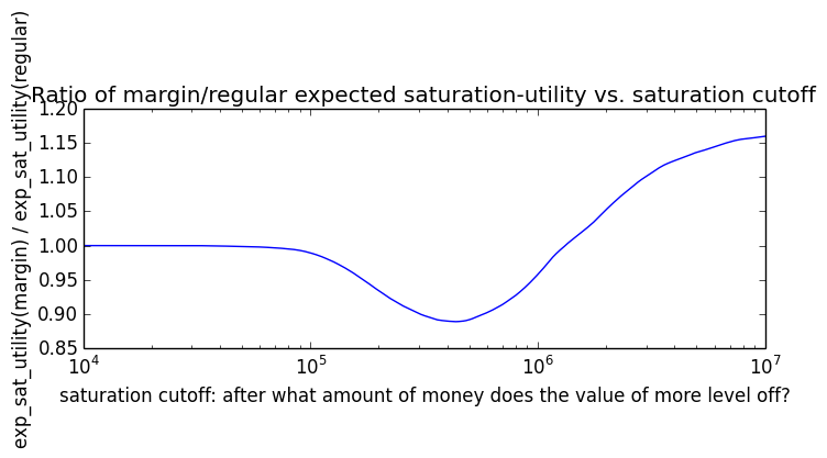
Here's how the expected utility of regular vs. margin investing compare if utility(wealth) = (wealth)α for 0 ≤ α ≤ 1: If we instead assumed that wealth had linear value up until some saturation point (expressed in present value of $), after which it stopped being useful, we'd instead have this graph for expected saturation-utility:
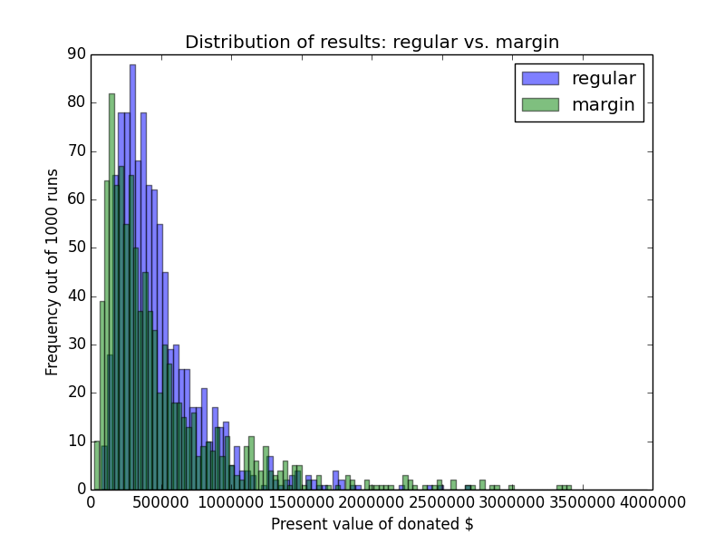
Calculations of expected utility given some α parameter may be overly abstract, so it's also helpful to ground one's intuitions in a basic histogram of outcome possibilities. This graph shows the distribution of ending wealth for regular vs. margin investing. With which distribution of results would you be able to do more expected good via your donations?
Graphs of interest
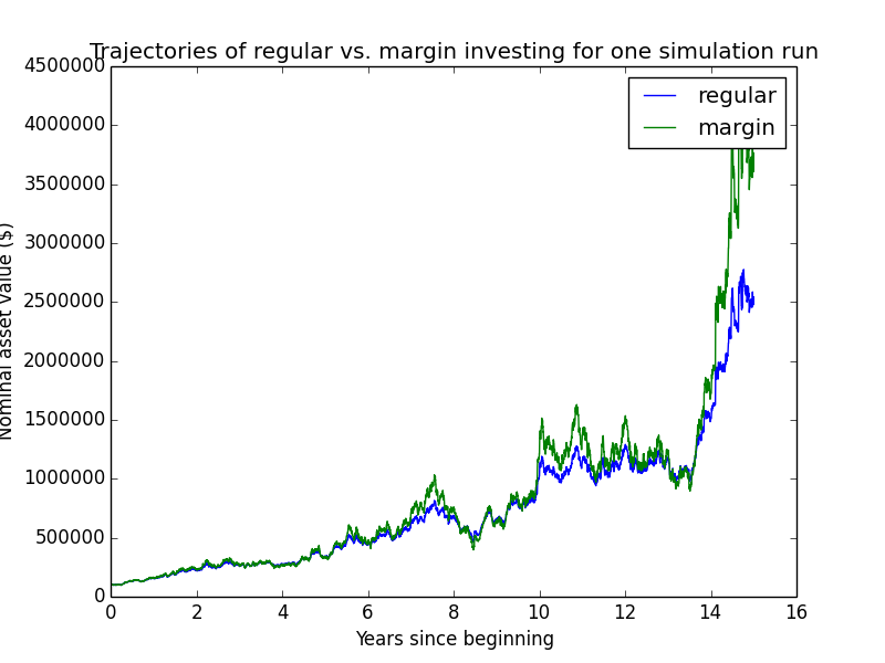
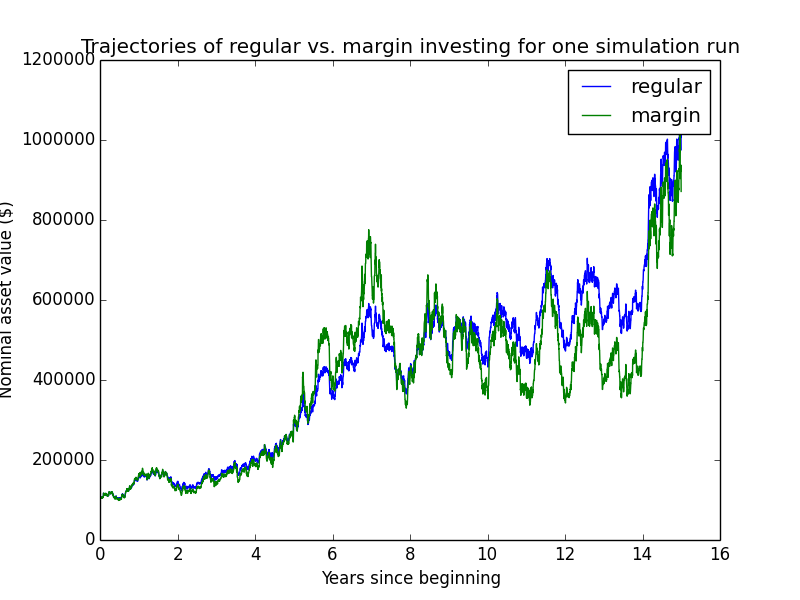
Here are some individual trajectories of the two account types. We can see that margin usually underperforms regular.
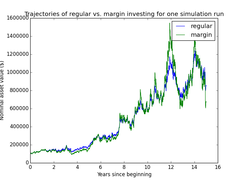
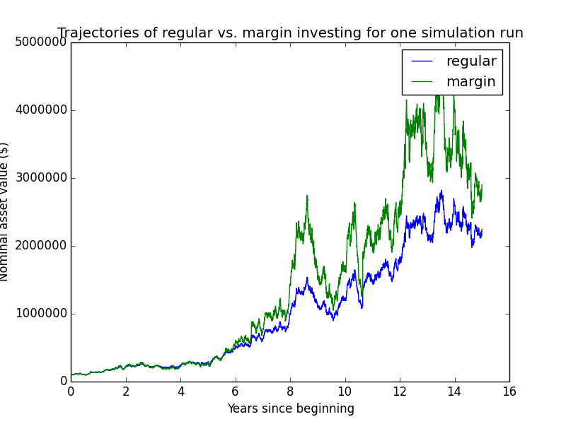
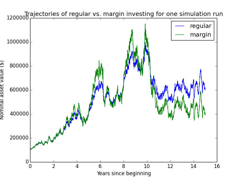
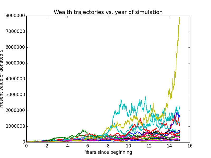
The next chart shows (real present value) wealth trajectories for the first 20 individual runs of the simulation. Each colored line is one history of the investor under some configuration of market performance and unemployment outcomes.
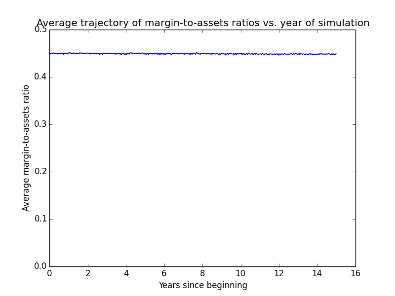
An investor's margin-to-assets ratio is debt/(total securities value). For example, if you start with $5 and borrow another $5 to buy $10 of an ETF, your margin is $5 and assets are $10, giving a margin-to-assets ratio of .5. The following graph shows the average progression of the simulated investors' margin-to-assets ratios over time. .45 is the target leverage when buying new securities.
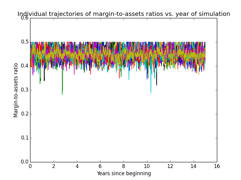
And this graph shows individual trajectories for the first 20 random investors' margin-to-assets ratios.
Since the investor sells the biggest capital losses, both for tax-loss harvesting and when she needs money for rebalancing, she accumulates capital losses over time, of which she can deduct $3K per year from income taxes. Following are the first 20 random trajectories of how much capital loss is accumulated over time:
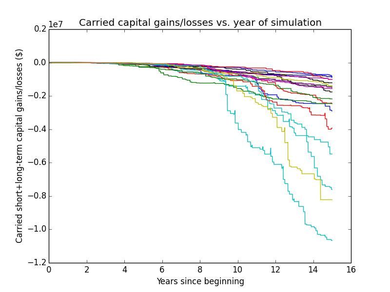
The numbers are quite high (~$1 million for a typical run). Part of the reason for this is that these numbers aren't discounted the way the final results are. Nominal asset values for the accounts tend to be at least ~$1 million in a given year. Say asset values go up or down ~1% on average each day, and every other day the values go down. Then every other day, there's a $10K capital loss. If all of those losses could be harvested without also catching capital gains in the process (which of course isn't true), then an investor could accumulate $1 million of capital losses within 200 days. So it doesn't seem out of the question that an investor could in practice accumulate $1 million of capital losses over 15 years.
This next graph shows how much the actual simulated margin-account values deviate from what one would compute using a very simple constant-leverage calculation, for the first few individual trajectories of the simulation. The graph serves two purposes:
- verifying that the complex simulation isn't going too far awry due to undiscovered bugs
- showing how much difference the complexities of the simulation make to the overall result.
I only needed to plot margin-account values because non-margin-account values perfectly match a simple calculation.
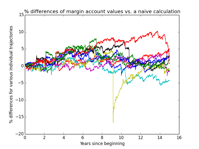
Based on how small these differences usually are, it looks like I probably could have made my simulation a lot simpler without much loss of accuracy! But it's already written, so I'm using it.
Input parameters for these results:
The following parameters are what I refer to as the "default" settings in the rest of this essay:
- invest for 15 years before donating
- after-tax savings are $30,000/year in the first year, with 2% real annual growth (i.e., after 15 years, inflation-adjusted savings are about $40,376/year), with a slight penalty the more times the person is laid off
- starting emergency money, which gets invested without leverage, is $100,000
- short-term capital-gains tax rate = 0.28
- long-term capital-gains tax rate = 0.15
- state income-tax rate (whether short-term or long-term gains) = 0.05
- monthly probability of being laid off = 0.01
- monthly probability of finding work after being laid off = 0.2
- average annual returns (continuously compounded) of index ETF = 5.4% (This assumes a return of 5.6% not continuously compounded, since ln(1 + 0.056) = 0.054. This estimate is conservative, since historical returns have been more like ~10% in the US, but historical US returns are probably too high because of selection biases. The reason to use continuous interest is that stock prices are compounded daily 252 times per year, so the return is approximately continuously compounded anyway. To see this, note that (1+[ln(1.056)]/252)252 ≈ 1.056.)
- annual volatility of index ETF = 22% (I calculated this based on SPY data from 3 Jan. 2007 to 2 Apr. 2015. You could also look at the VIX index. That said, I don't recommend investing in the US stock market at the moment because some think it's overpriced. So I picked a random global index ETF, ACWI, and found that it had annual volatility of 0.24 between 28 Mar. 2008 to 1 May 2015, which is close enough to my parameter setting. ACWI has about 50% holdings in the USA. It would be good to look at volatility for other types of index ETFs too.)
- "medium black swan" probability = 0.004
- annual volatility for "medium black swan" event = 1.1
- "large black swan" probability = 0.0001
- annual volatility for "large black swan" event = 4.1
- trading days per year = 252
- margin interest rate = 3.0% (The actual current margin rate on Interactive Brokers is 1.12% for account balances of at least $100K and less than $1M. I chose a higher value of 3.0% to make the calculations more conservative and because current interest rates are extremely low by historical standards, which is a trend that may not last for 15 more years. The effective margin interest rate is also lower if you deduct margin interest payments against other net investment income. To keep things conservative, I ignore this point, since you may not have much other net investment income. If you're buy-and-hold investing to donate appreciated securities, the only investment income you'd have would be from dividends, not from capital gains.)
- inflation rate = 3.0% (see p. 5 of this piece)
- broker-imposed max margin-to-assets ratio in your margin account = 50% (This is unrealistically low for Interactive Brokers, and if I were doing the simulation over, I would have increased it. Also, for simplicity, I'm not distinguishing initial margin vs. maintenance margin.)
- voluntarily self-imposed max margin-to-assets ratio in the account = 45% (The investor does voluntary monthly rebalancing to keep margin below this ratio.)
- trading fee per dollar of securities bought or sold = $0.000285 (this counts both Interactive Brokers trading fees and bid-ask spreads)
- number of random iterations = 1000
Explanation of "black swan" probabilities
Simple stock-market models typically use geometric Brownian motion. This is fine for some purposes, but when considering long-term leverage investing, the fat tails of actual financial distributions become important. "Leveraged Canadian Stock Portfolios: Long-Run Effects on Wealth and Risk" notes that a 4X leverage strategy would have done badly between 1950 and 2001. One reason was 1987's Black Monday, which would have almost wiped out the whole margin account balance due to a one-day loss of ~23%. (Even end-of-day rebalancing wouldn't have been able to prevent losing almost all account value.) Clearly, "black swan" events like these can make a big difference to the final analysis.
The parameters of my normal distribution are μ = 0.054 and σ = 0.22. Consider a one-day market movement. Assuming 252 trading days per year, the expected daily movement is 0.054/252 = 0.00021, and the standard deviation is 0.22 / √252 = 0.014. Since the standard deviation is so much bigger than the mean, let's just focus on the standard deviation and assume a mean of 0.
A loss of 23% in a single day (Black Monday) means multiplying previous prices by (1-0.23). Since geometric Brownian motion implies continuous compounding, we should convert this to a continuous rate. We want a change C such that exp(C) = 1-0.23, which means C = ln(1-0.23) = -0.26. This is a daily return that should be able to be sampled from our distribution of daily returns—the distribution with a mean of (roughly) 0 and a standard deviation of 0.014. But the z-value for a -0.26 return is -0.26/.014 = -19, which has a probability so small that online normal-distribution calculators can't handle it. Basically, this event should have never happened. But it did once over the 51-year period from 1950 to 2001. This needs to be addressed in the simulations or else they risk ignoring huge risk from black swans.
There are many proposals for modeling fat-tailed distributions in finance. To keep things simple, I chose a finite mixture of normal distributions (see section 6.3 of this paper). I estimated the parameters by hand in a quick-and-dirty way as described below, but of course it would help to use more systematically determined parameters, as well as to try other fat-tailed distributions.
Also note that there's a bit of double counting in that for non-black-swan days, I'm using a volatility estimate based on long-run daily-return data, which include some highly volatile periods. Ideally I would exclude the black swans from the data when calculating the non-black-swan mean and variance, but I assume the difference this would make is small, and neglecting to do it just makes the calculations more cautious.
I looked at Wikipedia's "List of largest daily changes in the Dow Jones Industrial Average", focusing on the largest percentage changes. The dates go back to 1898. The range from 1898 to 2014 is 116 years. Multiplying by 252 trading days per year, that's roughly 30,000 days. I copied the changes into a spreadsheet and computed the equivalent continuous-compounding daily returns.
Except for Black Monday, the returns are relatively uniform, but a normal approximation will do. The standard deviation of the 39 returns excluding Black Monday is about 0.09, but this estimate is inflated because my data set includes numbers like -0.07 and +0.07 but no numbers like -0.02, 0, or +0.02 (i.e., the middle of the distribution is empty). Instead, I estimated the standard deviation by eye. The numbers with the smallest magnitudes in the data set are about -0.07 and +0.07. Say that's one standard deviation from an assumed mean of 0. Then -0.14 and +0.14 would be two standard deviations from 0. Observations that extreme or more should occur 5% of the time, and indeed, we see two data points out of the 39 that are roughly 0.14 in magnitude. Now, the 39 numbers are missing data within one standard deviation of 0. About 68% of observations fall within one standard deviation of the mean. So we can assume that the 39 data points correspond to 100%-68% = 32% of all instances of returns drawn from this distribution. In other words, we can imagine there were 39/.32 = 122 events drawn from this distribution in total, out of 30,000 total days. So the probability that a given daily return will be drawn from this distribution out of the mixture of normals is 122/30,000 = 0.004. Finally, note that the standard deviation of 0.07 is for one day, which means the annualized volatility would be 0.07 * √252 = 1.1. These are the parameters I used for medium-scale black swans.
Now to handle Black Monday. Suppose that it was 1 standard deviation from the mean of a large-scale black swan distribution. That implies the daily volatility for this distribution is 0.26, which annualizes to 0.26 * √252 = 4.1. It happened once in 30,000 days, so the probability of drawing from this distribution is 0.00003. To make the calculations more conservative and help account for black-swan changes more extreme than anything we've seen before, increase the probability threefold to 0.0001. In other words, the probability that a 15-year investing period hits at least one such event is 1-Prob(hit zero of them) = 1-0.9999(15 * 252) = 0.31.
I implemented the mixture of normal distributions by picking a random floating-point number between 0 and 1. If it was <.0001, I used the extreme black-swan distribution. If it was between 0.0001 and 0.0041, I used the medium black-swan distribution. Otherwise I used the default normal distribution.
How the simulation works
I compare investing in a regular brokerage account vs. buying on margin. In both cases, I assume you only buy a single index ETF.d Its price updates every weekday. You get paid every month and use that new income for investing. If you have a margin account, you also pay interest on it every month, on your pay day.
Most of the time you're earning money, but occasionally, at random, you might get laid off. I incorporated this aspect of the simulation to make calculations more conservative. The idea came from this post. In fact, that post suggests that layoffs are more likely during market downturns, but for simplicity, I made layoffs just random.
If you use a regular brokerage account, then every month when you're not laid off, you just use your new income to buy more of the index ETF. End of story.
If you use a margin account, your actions are a bit more complex. With the money that you earn when you're not laid off:
- First you pay whatever interest is due on your margin borrowing from prior months, using the new savings that you're depositing. (If you don't have enough income this month to cover interest, you sell some of your investments to pay the interest. In the simulations I've run, this only happens when you get laid off.)
- You check the margin-to-assets ratio in your margin account. If it's below 45% (i.e., 90% of the broker-required 50% ratio), you leave the account alone. If the margin-to-assets ratio is above 45%, you first pay for it with that month's paycheck, and if that's not enough, you sell some investments to bring the ratio back down to 45%. It may be best not to do this too much because selling investments can incur capital-gains tax. That said, one of two cases where your margin-to-assets ratio gets above 45% is when the market underperforms the interest rate, which means you tend to have capital losses and so get some tax benefit from selling. The program chooses the most tax-advantaged lots of your portfolio to sell, based on which, if sold, would trigger the least capital-gains tax (which includes the biggest negative capital-gains tax if you have losses). The other case where your margin-to-assets ratio might get too big is if you're laid off for more than a brief period, so that interest payments pile up.
- If you have any monthly income left over after the previous steps, use it to buy new shares of the index ETF at a margin-to-assets ratio of 45%, i.e., for every $100 of shares you buy directly, you also loan $81.82 to buy more shares on margin. This is because 81.82 / (81.82 + 100) = .45.
- If your margin-to-assets ratio is below our target (45%), then buy new securities to reach your target. In order to avoid incurring transactions costs on trivially small equity purchases, you only buy new ETF shares for rebalancing if you can buy at least $50 of such shares at once.
As you move toward your target date for donating the securities, you ramp down leverage to make sure you'll have enough equity to pay off your debts. This ramp-down basically doesn't affect the default scenario of 2X leverage, but for higher leverage amounts, it forces you to drop down to being within 3X leverage when there are at most 10 years left and within 2X leverage when there are at most 5 years left.
You maintain a self-imposed maximum margin-to-assets ratio of 45% to give some breathing room relative to the broker-imposed maximum margin-to-assets ratio of 50%. In the simulation, the broker checks the margin-to-assets ratio every weekday and, if it's above 50%, sells securities randomly to keep the ratio within bounds. But this is bad for you, since it leads to unpredictable selling behavior. For instance, maybe the broker sells securities with high, short-term capital gains rather than those with capital losses. It's better if you can personally keep margin-to-assets ratios in check by selling securities manually as needed. But you don't want to manage the account daily, so you monthly keep the margin-to-assets ratio less than 45%, on the assumption that the ratio won't move above 50% within the next month. Adopting this policy reduces manual maintenance work. It's much easier to check a margin account 12 times a year than 252 times a year, and the lost leverage by maintaining a maximum 45% ratio instead of 50% isn't that big.
Different variations of a margin strategy sell securities at different rates. The more leveraged you are, the more likely you are to sell securities at a loss to meet margin requirements. This means some strategies get more tax benefit from capital losses than others. To help put the strategies on somewhat more even footing, I added tax-loss harvesting, which is done by both margin and regular investors every December: You sell all securities with losses and use the money to buy the sold ETF back. (In real life, you'd have to wait a month before buying back to avoid a wash sale, but in the simulation you buy it back immediately for simplicity.)e
Your capital-gains taxes accumulate from selling, both for tax-loss harvesting and for rebalancing your margin account as needed. Every March 1, you pay off any taxes owed, if necessary by selling some securities. However, almost uniformly you have net capital losses, because basically the only times you might sell securities at a capital gain are (1) if the broker liquidates them to keep you within the 50% margin limit or (2) if you're unemployed for a while and have to sell ETF shares with gains.
The simulation assumes the investor starts off with emergency funds that are only invested without leverage. Having emergency funds makes sense in case you need money urgently after your margin account has gone bust. Some possible reasons why you might need money urgently:
- you get laid off for a while
- a parent, spouse, friend, etc. needs a big loan urgently
- you want to quit your job early and don't have enough in your 401k to retire on
- you come across an altruistic project that requires donations now or never and has such high value that you can't afford not to donate immediately.
The invested value of emergency funds is counted as part of your total invested money at the end of the simulation. I count the emergency money toward your total donation amount, which would make sense if the end of the simulation corresponds to your retirement, at which point you can donate the emergency funds and live off your 401k. Alternatively, we can interpret the utility(wealth) = (wealth)α utility function to represent both your own living expenses and what you donate to charity beyond personal costs of living, in which case it makes sense to include emergency funds as part of the wealth input to this utility function even if you'll spend those funds on yourself rather than donating them. f
In rare cases, such as when a big negative black swan occurs, highly leveraged accounts might get wiped out due to having more debt than remaining assets. If that happens, you tap into your emergency savings. There are two possibilities:
- If emergency savings are enough to pay off the shortfall, then you pay off your debts. Then with future salary, you restore your emergency fund until it's equal with what it would have been had you not invested on margin. After that, you continue margin investing as usual.
- If even emergency savings can't cover the shortfall, you pay off what you can and go completely broke, declaring bankruptcy to eliminate your debts. After that, I assume that your ability to get credit is so bad that you can't invest on margin anymore (I'm not sure if this is true in practice??), so you just invest future earnings in regular equities without leverage thereafter.
When you're ready to donate your securities, you use your investments to pay off any remaining margin loans. Because you're donating the final securities, there's no capital-gains tax on them. If instead you use this calculator for personal investing (say, for retirement) rather than investing prior to donating, then you'd need to account for capital-gains tax upon selling. (In that case, it's less bad to pay capital-gains taxes early because doing so increases your cost basis, though it's still better to delay tax payments to later years because of the time value of money.)
The final comparison among the strategies as presented in the results is the present value of accumulated savings, i.e., the value after t years times exp(-μt) to make it a present value. Looking at present values is more informative than future values because we have a better sense of what the value of a dollar is right now than what the value of a dollar will be in 15 years.
It's unclear what discount rate I should have used:
- I chose μ because this represents the opportunity cost of delayed investing for a risk-neutral investor who would have invested in regular equities.
- I could also have used something closer to r to represent a risk-free rate of return, which is standard in most present-value calculations.
- Finally, I could have used the rate of return of the activities of the charity to which the donor will be giving plus the rate of return on the donor's wisdom from giving later, since that represents the opportunity cost of waiting until later to give.
Fortunately, the discount rate doesn't affect the ratio of performance between regular vs. margin investing, just the magnitudes of absolute ending wealth.
The simulation seeds the random-number generator used for market and unemployment randomness at the same value across all variations that I ran. This helps reduce noise when making comparisons across variants because different variants are being evaluated against the same series of market and unemployment outcomes. Using a seed also helped with debugging, because I could precisely reproduce any weird behavior that I saw and could compare two variants side by side to look for where they diverged due to non-random factors.
Results vs. theory
The simulation discussed above has many real-world complexities. Theoretical academic formulas for margin returns are much simpler. As a way to check that my complicated simulation was roughly on the right track, I ran a version of the simulation in which lots of complicating factors were ignored. In particular:
- no unemployment, inflation, taxes, black swans, or emergency funds
- the investor gets paid on only one occasion—namely, her first pay period right when the simulation starts
- the investor rebalances monthly toward a leverage ratio exactly equal to the broker-imposed leverage limit rather than comfortably under that limit as in the default scenario
- the investor doesn't taper off leverage toward the end of the investing period.
Following are the results with this much simpler version of the simulation:
| Type | Mean ± stderr | Median | Min | Max | E[√wealth] ± stderr | σln(wealth) |
| Regular | $2,448 ± $85 | $1,676 | $171 | $46,213 | 45 ± 1 | 0.86 |
| Margin | $3,666 ± $594 | $847 | $10 | $550,301 | 42 ± 1 | 1.66 |
| Regular + 50% match | $3,672 ± $127 | $2,515 | $257 | $69,319 | 55 ± 1 | 0.86 |
Leverage is better than regular 21% of the time. Margin investor ended with no assets and a deficit in emergency savings 0.0% of the time. Leveraged account went fully bankrupt 0.0% of the time. Average simple-calculation margin ending balance was $3,704.

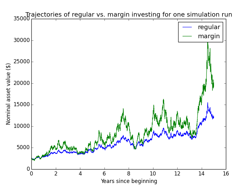
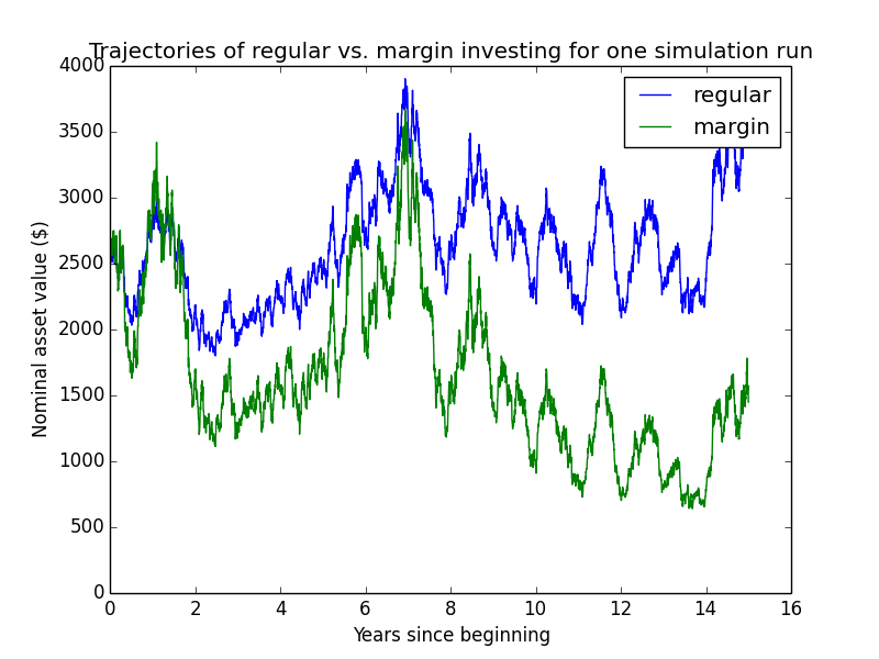

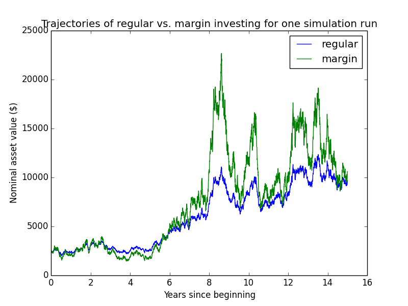
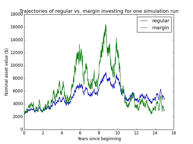
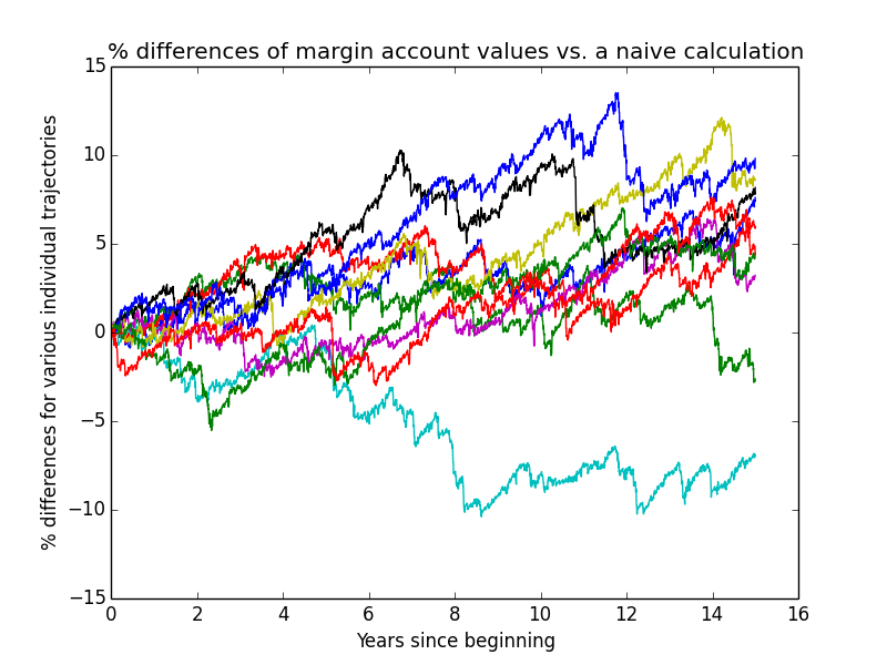
I compare these numbers with theory below.
Validating the results of regular investing
Median wealth
The theoretical median outcome for regular investing is shown in the regular median equation. However, when I reported my numbers in this simulation, I discounted final wealth using continuous compounding at a discount rate of μ = 0.054 per year over a time of t = 15 years. That is, I multiplied the final amounts by exp(- 0.054 * 15). Multiplying the regular median equation by this factor gives S0 exp(μt - σ2t/2) exp(-μt) = S0 exp(-σ2t/2). This is what we predict the median simulation outcome will be.
In the simulation, I used t = 15 years, μ = 0.054 per year, σ = 0.22, and S0 = $2,466. The empirical median from the above table, $1,676, is very close to the theoretical value, $2,466 exp(-0.222 * 15/2) = $1,715.
Mean wealth
We found the theoretical mean above in regular mean equation. When discounted, it becomes S0 exp(μt) exp(-μt) = S0, i.e., just the initial price. So the theoretical mean is just the initial amount invested: $2,466. The empirical mean value from the above table is $2,448 ± $85.
Std dev of log wealth
If we take ln of both sides of the regular St equation, we get
ln(St) = ln(S0) + μt - σ2t/2 + σWt.
The only randomness here is in Wt, so
StdDev[ln(St)] = StdDev[σWt] = σStdDev[Wt] = σ√t = 0.22 * √15 = 0.85.
In the simulations, I found StdDev[ln(St)] = σln(wealth) = 0.86 for regular investing, which is again pretty close.
Validating the results of margin investing
Median wealth
Discounting the leveraged median equation:
- Theoretical discounted median = V0 exp{(r + (μ-r)c) t - c2σ2t/2} exp(-μt) = V0 exp{(rt + μct - μt - rct - c2σ2t/2} = V0 exp{μ(c-1)t - r(c-1)t - c2σ2t/2} = V0 exp{(μ-r)(c-1)t - c2σ2t/2} = $2,466 * exp{(0.054-0.03) * (2.0-1) * 15 - 2.02 * 0.222 * 15/2} = $827
- Empirical discounted median = $847
Mean wealth
Discounting the leveraged mean equation:
- Theoretical discounted mean = V0 exp{(r + (μ-r)c) t} exp(-μt) = V0 exp{rt + μct - μt - rct} = V0 exp{μ(c-1)t - r(c-1)t} = V0 exp{(μ-r)(c-1)t} = $2,466 * exp{(0.054-0.03) * (2.0-1) * 15} = $3,534
- Empirical discounted mean = $3,666 ± $594
Std dev of log wealth
Taking ln of both sides of the leveraged Vt equation:
ln(Vt) = ln(V0) + (r + (μ-r)c) t - c2σ2t/2 + cσWt.
The only randomness here is in Wt, so
StdDev[ln(Vt)] = StdDev[cσWt] = cσStdDev[Wt] = cσ√t = 2.0 * 0.22 * √15 = 1.7.
The empirical value of σln(wealth) for margin investing in the above table was 1.66.
Prob[margin beats regular]
We want to know the probability that margin investing does better than regular, Prob[Vt > St], on the same underlying asset trajectory. Assume both portfolios start out with equal initial capital: V0 = S0 = K. Then, using the regular St equation and leveraged Vt equation:
= Prob[ln(K) + (r + (μ-r)c) t - c2σ2t/2 + cσWt > ln(K) + μt - σ2t/2 + σWt]
= Prob[(r + (μ-r)c) t - (c2-1)σ2t/2 + (c-1)σWt > μt]
= Prob[r + (μ-r)c - (c2-1)σ2/2 + (c-1)σWt/t > μ]
= Prob[(1-c)r + μ(c-1) - (c2-1)σ2/2 + (c-1)σWt/t > 0]
= Prob[(μ-r)(c-1) - (c2-1)σ2/2 + (c-1)σWt/t > 0]
= Prob[(c-1)σWt/t > (c2-1)σ2/2 - (μ-r)(c-1)]
= Prob[(c-1)σWt/t > (c-1)(c+1)σ2/2 - (μ-r)(c-1)]
= Prob[σWt/t > (c+1)σ2/2 - (μ-r)]
= Prob[Wt/t > (c+1)σ/2 - (μ-r)/σ].
Now recall that if Z is a standard-normal random variable, Wt = Z√t. Substituting in:
= Prob[Z > √t( (c+1)σ/2 - (μ-r)/σ )]
= 1 - Prob[Z ≤ √t( (c+1)σ/2 - (μ-r)/σ )]
= 1 - Prob[Z ≤ √15( (2.0+1)0.22/2 - (0.054-0.03)/0.22 )]
= 1 - Prob[ Z ≤ 0.86 ]
= 1 - 0.8
= 0.2.
The empirical probability of margin outperforming regular investing in the above table is 21%.
Note that this probability gets smaller as t increases because √t( (c+1)σ/2 - (μ-r)/σ ) is √t times a positive number. But if the parameters were somewhat different, this probability would actually increase with bigger t. That would happen if and only if
(c+1)σ/2 < (μ-r)/σ
c < 2(μ-r)/σ2 - 1.
The expression (μ-r)/σ2 will show up later as being the Kelly-criterion optimal amount of leverage. So this expression says that leverage tends to beat regular investing with longer time horizons when the actual leverage amount, c, is no more than 2 * (Kelly-optimal leverage amount) - 1.
Relaxing the simplifying assumptions
When doing this empirical validation, I ran the simulation with many complicating factors ignored in order to better match theory. This section shows how the results change as the complicating factors are gradually added back in, until eventually we arrive back at the complicated, "default" configuration.
From simple scenario, relax assumption of only earning one initial paycheck
| Type | Mean ± stderr | Median | Min | Max | E[√wealth] ± stderr | σln(wealth) |
| Regular | $349,434 ± $6,653 | $297,951 | $85,257 | $2,647,212 | 571 ± 5 | 0.51 |
| Margin | $435,369 ± $28,276 | $237,411 | $30,983 | $21,589,872 | 571 ± 10 | 0.93 |
| Regular + 50% match | $524,152 ± $9,979 | $446,927 | $127,885 | $3,970,817 | 699 ± 6 | 0.51 |
Leverage is better than regular 30% of the time. Margin investor ended with no assets and a deficit in emergency savings 0.0% of the time. Leveraged account went fully bankrupt 0.0% of the time. Average simple-calculation margin ending balance was $437,904.
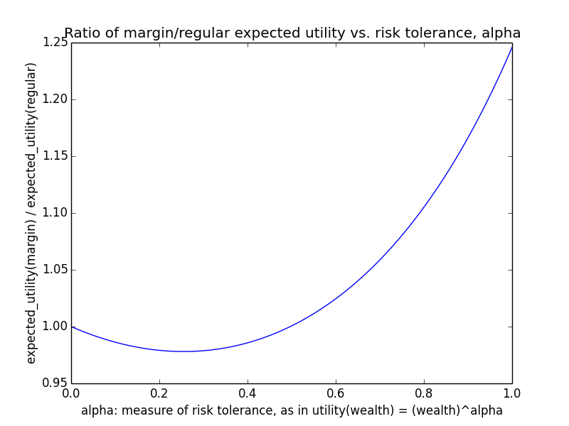
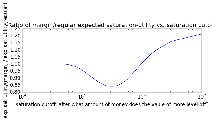
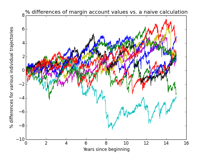
From that, relax assumption of maintaining leverage equal to broker max
| Type | Mean ± stderr | Median | Min | Max | E[√wealth] ± stderr | σln(wealth) |
| Regular | $349,434 ± $6,653 | $297,951 | $85,257 | $2,647,212 | 571 ± 5 | 0.51 |
| Margin | $419,141 ± $22,986 | $248,601 | $35,301 | $16,761,148 | 572 ± 10 | 0.88 |
| Regular + 50% match | $524,152 ± $9,979 | $446,927 | $127,885 | $3,970,817 | 699 ± 6 | 0.51 |
Leverage is better than regular 31% of the time. Margin investor ended with no assets and a deficit in emergency savings 0.0% of the time. Leveraged account went fully bankrupt 0.0% of the time. Average simple-calculation margin ending balance was $418,296.

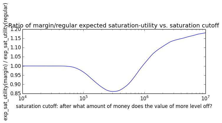
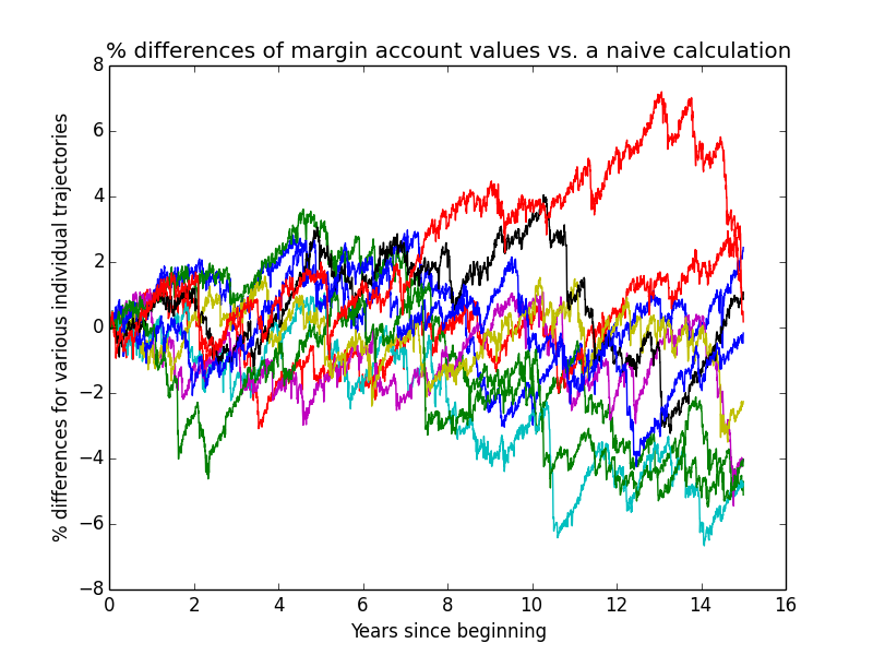
From that, relax assumption of not tapering off leverage toward end
| Type | Mean ± stderr | Median | Min | Max | E[√wealth] ± stderr | σln(wealth) |
| Regular | $349,434 ± $6,653 | $297,951 | $85,257 | $2,647,212 | 571 ± 5 | 0.51 |
| Margin | $419,141 ± $22,986 | $248,601 | $35,301 | $16,761,148 | 572 ± 10 | 0.88 |
| Regular + 50% match | $524,152 ± $9,979 | $446,927 | $127,885 | $3,970,817 | 699 ± 6 | 0.51 |
Leverage is better than regular 31% of the time. Margin investor ended with no assets and a deficit in emergency savings 0.0% of the time. Leveraged account went fully bankrupt 0.0% of the time. Average simple-calculation margin ending balance was $418,296.
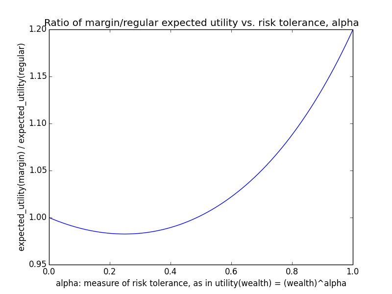


From that, relax assumption of no black swans
| Type | Mean ± stderr | Median | Min | Max | E[√wealth] ± stderr | σln(wealth) |
| Regular | $350,149 ± $7,208 | $291,437 | $54,854 | $2,712,839 | 568 ± 5 | 0.55 |
| Margin | $422,711 ± $24,245 | $233,241 | $8,191 | $16,629,383 | 565 ± 10 | 0.94 |
| Regular + 50% match | $525,223 ± $10,812 | $437,155 | $82,281 | $4,069,259 | 696 ± 6 | 0.55 |
Leverage is better than regular 28% of the time. Margin investor ended with no assets and a deficit in emergency savings 0.0% of the time. Leveraged account went fully bankrupt 0.0% of the time. Average simple-calculation margin ending balance was $421,241.

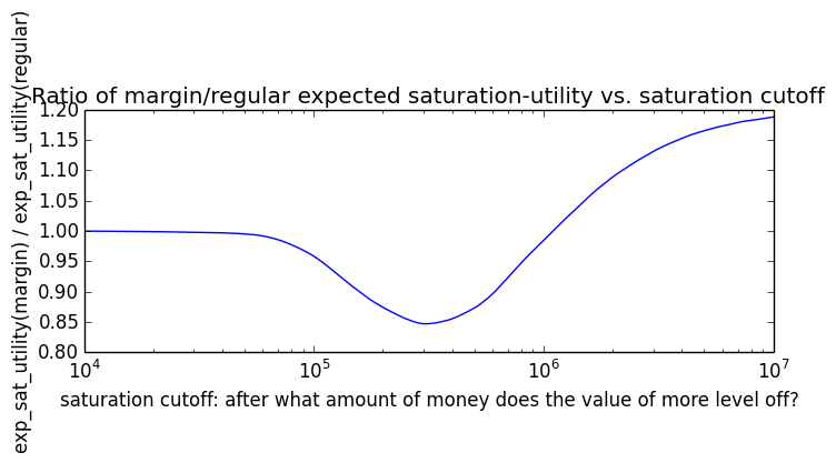
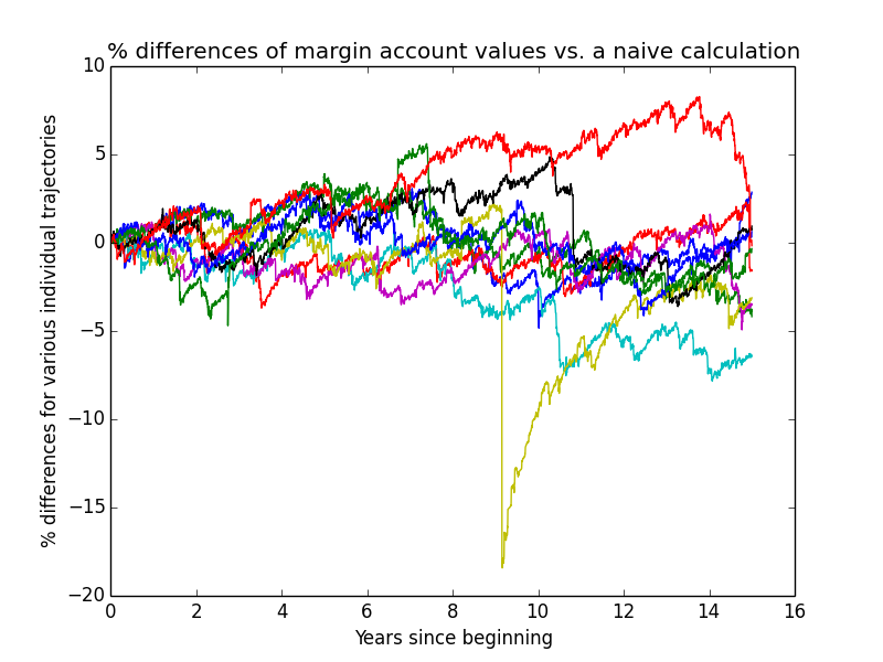
From that, relax assumption of no taxes
| Type | Mean ± stderr | Median | Min | Max | E[√wealth] ± stderr | σln(wealth) |
| Regular | $350,149 ± $7,208 | $291,437 | $54,854 | $2,712,839 | 568 ± 5 | 0.55 |
| Margin | $433,078 ± $24,705 | $239,558 | $8,758 | $16,861,620 | 572 ± 10 | 0.94 |
| Regular + 50% match | $525,223 ± $10,812 | $437,155 | $82,281 | $4,069,259 | 696 ± 6 | 0.55 |
Leverage is better than regular 32% of the time. Margin investor ended with no assets and a deficit in emergency savings 0.0% of the time. Leveraged account went fully bankrupt 0.0% of the time. Average simple-calculation margin ending balance was $421,241.
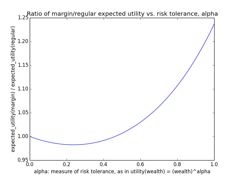
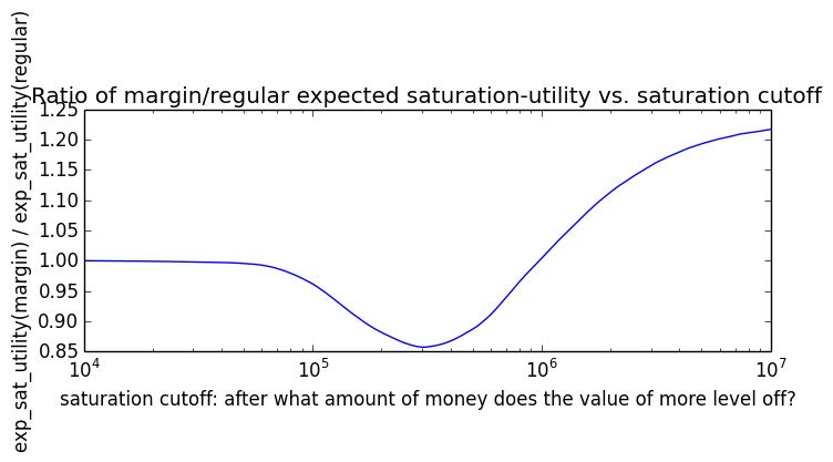
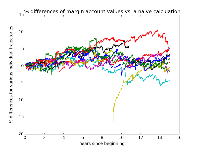
From that, relax assumption of no inflation
| Type | Mean ± stderr | Median | Min | Max | E[√wealth] ± stderr | σln(wealth) |
| Regular | $425,839 ± $8,249 | $359,356 | $78,803 | $3,001,729 | 629 ± 5 | 0.52 |
| Margin | $518,129 ± $27,249 | $299,267 | $11,937 | $17,947,707 | 634 ± 11 | 0.89 |
| Regular + 50% match | $638,759 ± $12,374 | $539,034 | $118,204 | $4,502,593 | 771 ± 7 | 0.52 |
Leverage is better than regular 32% of the time. Margin investor ended with no assets and a deficit in emergency savings 0.0% of the time. Leveraged account went fully bankrupt 0.0% of the time. Average simple-calculation margin ending balance was $506,209.
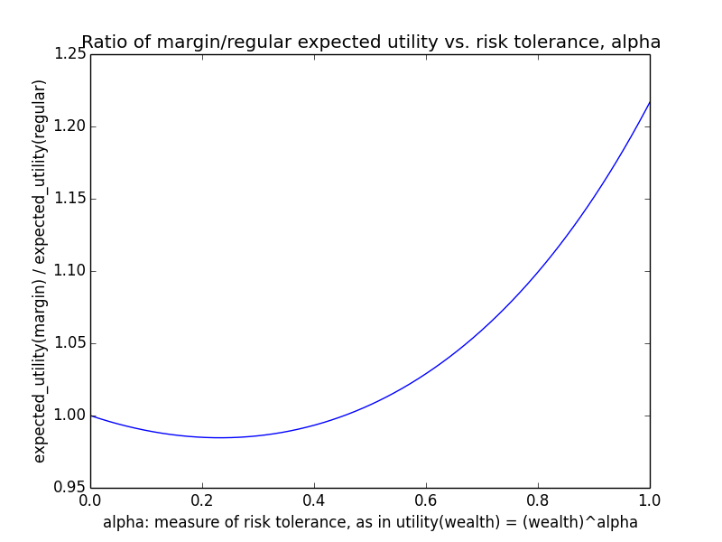
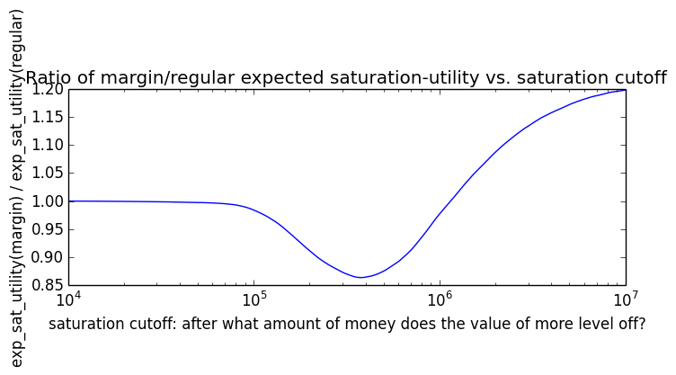
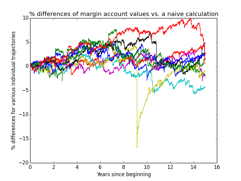
From that, relax assumption of no unemployment
| Type | Mean ± stderr | Median | Min | Max | E[√wealth] ± stderr | σln(wealth) |
| Regular | $387,985 ± $7,688 | $328,643 | $73,896 | $2,612,862 | 599 ± 5 | 0.53 |
| Margin | $474,319 ± $25,047 | $270,926 | $11,255 | $16,106,461 | 604 ± 10 | 0.91 |
| Regular + 50% match | $581,977 ± $11,532 | $492,964 | $110,844 | $3,919,293 | 734 ± 7 | 0.53 |
Leverage is better than regular 33% of the time. Margin investor ended with no assets and a deficit in emergency savings 0.0% of the time. Leveraged account went fully bankrupt 0.0% of the time. Average simple-calculation margin ending balance was $462,480.

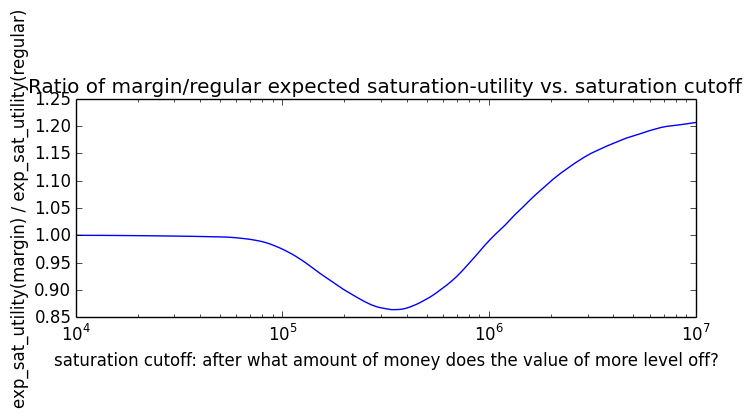

The only assumption left here is that of no emergency funds. Relaxing this assumption too would bring us back to the results table for the "default" parameter configuration discussed earlier.
401k matching beats leverage
Lifecycle Investing points out that most 401k plans don't allow leverage. IRAs in general don't allow margin debt for the most part. But many employers match 401k contributions at a 2X or 1.5X rate. Lifecycle Investing says you should always max out matching 401k contributions before investing with leverage on your own.
To test this out, I added to my simulation an investor who just contributed to a regular, non-margin brokerage account but was able to put in 50% more than normal. For instance, if regular investors contributed $2500/month, this investor contributed $3750/month. In practice, employers typically cap the amount of 401k contributions that can be matched per pay period at a relatively low level, but I ignored that point so that I could compare the 401k investor on equal footing with the other investors, and then if I saw the 401k investor beating the others, it would follow that any given dollar of employer-matched 401k investing would beat any given dollar of non-employer-matched margin investing, which would imply that you should max out employer matching first and only then use margin investing for the remaining income.
I did indeed find that a 50%-matched 401k beat either other type of investing. In fact, in the results vs. theory section, the 401k-matching strategy returned exactly 1.5 times the regular investing strategy, which it should have given that I compared the investments with respect to the same random stock-market returns. Because a 401k is tax-exempt, it might actually return more than 1.5 times a non-401k account if you sell investments and thereby incur extra capital-gains taxes in the non-401k account, but the non-401k account in this simulation had no capital-gains taxes because the wealth was donated at the end. (Note that 401k and non-401k investments can both be donated to charity tax-free.)
In reality, the amount you can contribute to a 50% matched 401k is more than 50% of what you can invest on margin on your own because a 401k is pre-tax, while margin investing uses post-tax dollars. However, you'll later have to pay taxes on your 401k withdrawals, so if your tax rate is the same now vs. in retirement, the tax-deferred nature of 401k contributions doesn't matter, since the amount at the end is (1-income_tax_rate) times (the pre-tax income that you put in plus equity appreciation). That said, if (as is common) you expect to have a lower marginal tax rate in retirement, this makes 401k contributing look even more favorable.
What about non-matched 401k?
The annual contribution limit for a 401k is $18K, which is probably higher than the amount that your employer matches. Should you only contribute to your 401k the amount your employer matches and invest the remainder in an after-tax margin account using leverage? Or should you contribute all $18K to the 401k and let the money grow tax-free there?
Reasons favoring 401k:
- If you expect to have enough income during retirement such that your capital-gains tax rate isn't 0%, you'd presumably pay ~15% taxes on capital gains outside a 401k, as well as possibly state income taxes on those capital gains, all of which would be avoided with a 401k.
- If you expect to be in a lower income bracket during retirement than your current income bracket (say 15% instead of 28%), then contributing to a 401k allows you to pay less income tax in addition to no capital-gains tax.
- Having some additional investments in a non-leveraged 401k could reduce your risk of a financial blow-up from using margin.
These factors combined seem pretty strong to me.
Reasons favoring margin investing:
- Perhaps you can get enough retirement savings just by the amount you contribute to your 401k for employer matching. In this case, you could donate your margin-invested securities and not pay capital-gains tax on them. If so, the only advantage of a 401k is that you might be in a lower income bracket during retirement.
- Currently, people in the 15% income bracket or below pay no capital-gains tax. So if your income during retirement was low enough, you might be able to spend your margin-invested savings on yourself without paying capital-gains tax. However, it might be hard to keep your income during retirement low enough to avoid paying capital-gains taxes, although you could presumably(?) donate excess 401k savings to ensure this. Likewise, it's quite possible that Congress will change capital-gains rates by the time of your retirement, so that even people in the 15% income bracket will pay capital-gains taxes.
- Contributing to a 401k locks the money in your retirement account for several decades. What if you want to donate it sooner? What if the financial system as a whole changes radically during those years, such that your 401k money becomes less valuable?
Leveraged ETFs in an IRA?
My impression is that it may be possible to buy leveraged ETFs in an IRA.(?) If so, if you have a 401k from a previous employer, you could convert it to an IRA and then buy leveraged ETFs in it. In this way, you'd get the benefits of employer matching and leverage combined.
Personally I probably won't leverage my 401k at this point because my future income stream is unclear, so I don't know for sure that I could replace the losses that might result from using leverage. If I were certain I'd be contributing to the 401k in a steady fashion for the next several decades, it would be more plausible that I should use leverage during my 20s and 30s in the manner that Lifecycle Investing suggests.
Donor-advised fund vs. leverage
As with a 401k, I don't think you can use leverage in a donor-advised fund (DAF). So should you forgo the DAF in order to use margin? The answer may depend on your situation.
How much is a DAF worth?
The advantage of a DAF is that you can deduct a donation from your income taxes immediately rather than when you eventually pick a charity to receive the funds.
If you donate small amounts
For small-time donors, deducting a donation now vs. later may not be crucial. Because of the time value of money, a given amount of tax deduction now is worth more than the same amount taken later. But if you wait until later, your funds to donate should in general have grown in value, so the value of deduction later will actually be larger, which roughly cancels the argument from time value of money for donating sooner.g So the value of DAF donating is roughly zero for these donors, ignoring other confounding factors such as that donating to a DAF may help maintain your commitment to donating but may also lock you in to donating to just US-based 501(c)(3)'s rather than other organizations or projects.
If you donate a lot
In contrast, donating to a DAF is quite important for big-time donors who plan to give at least 50% of adjusted gross income (AGI) each year. This is because donating every year helps these donors take full advantage of deductions, given that at most 50% of a person's AGI can be deducted for charity contributions in a single year. Charitable deductions above 50% carry forward to future years, but if you consistently donate above 50% every year, you'll never get a chance to take all your accumulated charity deductions. Hence, deducting charity donations each year that you earn becomes important.
If a donor in this situation doesn't have a charity picked out yet and would lose the year's charitable deductions if she didn't donate to a DAF, then donating to a DAF saves taxes. Say the donor is deep in the 28% marginal income bracket. By donating some amount $X (assume $X is below the 50%-of-AGI limit), she gets $.28X back on taxes (and that refund is untaxed), so it's as if she multiplied her money by 1.28. In other words, donating to a DAF is similar to donating to a 401k that matches 28% rather than 50%.
Whether this is better than leverage depends on the donor's risk tolerance and the advantage of leverage. For a risk-neutral investor, the DAF is better only if the expected wealth of using margin is less than 28% higher than not. For a risk-averse investor with utility(wealth) = √wealth, the DAF is better unless the E[√wealth] value in the above table is more than √1.28 times better for margin than non-margin (which it isn't). The reason for the √1.28 threshold is that donating to a DAF multiplies wealth by 1.28 with certainty, which means it multiplies expected √wealth by √1.28.
ESPP plans
A company's ESPP plan offers employees the opportunity to buy some amount of company stock at a discount (say, 10%). You should always participate in such programs, because if nothing else, you can just sell the stocks after you buy them (incurring taxes in the process). But it's better tax-wise to hold the securities for at least 2 years before selling or donating. [Update: ESPP shares involve tax complexities, so the time and effort required to figure taxes out should be weighed against the monetary savings you get on the share price.]
If you use margin investing, ESPP shares can just contribute to your assets, allowing you to borrow more. In contrast, if you use leveraged ETFs for leverage, then (non-leveraged) ESPP shares don't allow you to get leverage. In this case, you can trade off the tax penalty for selling the ESPP shares early (say, 14% or 28% income tax) against whatever percent benefit you see from investing that amount of money with leverage. If you agree with the philosophy of the investor in the simulations of keeping some non-leveraged emergency money, then ESPP shares could contribute toward that and hence would be compatible even with the approach of using leveraged ETFs.
Optimal leverage
In practice, margin leverage is not unlimited. But suppose it were. What would be the best amount of leverage to use?
Maximizing expected average return
In 2007, when I first learned about the capital allocation line, I saw that it suggests an investor could get arbitrarily high expected returns with arbitrarily high amounts of leverage. For a purely risk-neutral investor, this is a bonanza.
However, as Domian et al. (2003) explain: "In the single-period CAPM, expected return is an increasing linear function of the degree of leverage. But in our continuous time model, expected annualized return is a concave function of leverage." In fact, Domian et al. (2003) show that using c-times leverage (e.g., c = 2 means 2X leverage) and investing a fixed initial sum of wealth:
E[Rt] = r + (μ - r)c - σ2c2/2
where r is the borrowing interest rate, E[] indicates expected value, and
Rt := (1/t) ln(Vt/V0)
is the geometric-average t-year continuously compounded returnh, where Vt is the t-year accumulated wealth and V0 is the starting wealth.
Domian et al. (2003) show (eqn. 20, p. 7) that the leverage amount c* which optimizes E[Rt] is
c* = (μ - r)/σ2.
Using the parameter values for my default simulation, this optimal fraction is (0.054-0.03)/0.222 = 50%. Hence, this suggests using no leverage and splitting 50:50 between stocks and bonds! This isn't consistent with my results or with conventional wisdom. Of course, the parameters I used in this calculation were quite conservative. Based on historical US data, some people would set μ at more like .1, in which case the optimal betting fraction would be 1.45, i.e., almost 1.5X leverage.
The c* formula above corresponds to the Kelly criterion. This summary reviews how to derive the c* equation in a different way (p. 5). The Kelly criterion optimizes the growth rate of a portfolio with a single initial investment over the infinite future, i.e., R∞ using the above notation. This is equivalent to optimizing E[R1] because, by the strong law of large numbers, R∞ = E[R1] with probability 1. Since E[Rt] doesn't depend on t, what optimizes optimizes E[Rt] in general also optimizes E[R1].
Maximizing expected utility
While the Kelly criterion optimizes expected growth rate, that's not the same as optimizing expected ending wealth, and it's not the same as maximizing expected utility unless your utility function is the log of ending wealth.
Let u(Vt) be the utility of donating an amount Vt. Typically u is concave because additional dollars contribute less value. Also, in a world where other charity donations are highly correlated with yours based on market performance, if you get a lot of wealth because the market does well, other investors are also getting a lot of wealth, and hence, the value of a donate dollar isn't quite as high. For these reasons, I've used u(Vt) = √Vt in the results tables of this piece.
Case 1: utility(wealth) = ln(wealth)
For a given time horizon t, maximizing E[u(Vt)] is equivalent to maximizing E[u(Vt) - u(V0)], since V0 is a known constant. It's also equivalent to maximizing E{ (1/t) [u(Vt) - u(V0)] }, since t is a constant. Note that if u(Vt) = ln(Vt), then maximizing E{ (1/t) [u(Vt) - u(V0)] } means maximizing E[ (1/t) ln(Vt/V0) ] = E[Rt]. This is the Kelly optimization problem from before. So in this case, the Kelly criterion also optimizes expected utility.
But u(Vt) = ln(Vt) is a weird utility function. It places infinite disvalue on going bankrupt, since u(0) = ln(0) = -∞. Also, a logarithmic utility curve seems too pessimistic for an altruist, even considering the correlation of your returns with the returns of other donors, since there are still many valuable uses of money even in a richer world.
Case 2: utility(wealth) = wealth
Domian et al. (2003) prove the following equation (eqn. 14, p. 5), using the same variable meanings as in the previous section of their paper:
Vt = V0 exp{ [r + (μ-r)c - σ2c2/2 ]t + σcWt },
where Wt is a standard Brownian motion with mean 0 and annual variance t. Because Wt is normally distributed, Vt is lognormally distributed, and (eqn. 15, p. 5)
= V0exp{ [r + (μ-r)c]t },
where the extra σ2c2t/2 comes in because the mean of a lognormal distribution is greater than exp{the mean of the underlying normal distribution} because the exp{} function is convex.
The interesting thing about the equation for E[Vt] is that for μ > r, it's increasing in c, i.e., if you want to maximize expected ending wealth because E[u(Vt)] = E[Vt], then you should indeed partake of a leverage bonanza by maxing out leverage.
Case 3: utility(wealth) = (wealth)α
Suppose you have a risk-averse utility function but one that's not fully logarithmic like in the Kelly criterion. In particular, let utility(wealth) = (wealth)α. In the results tables of this piece, I've been taking α = .5, i.e., utility(wealth) = √wealth. Based on the formula for Vt, we have that
u(Vt) := Vtα = V0α exp{ [r + (μ-r)c - σ2c2/2 ]tα + σcWtα }.
Then, again using the fact about the mean of a lognormal distribution,
= V0α exp{ [r + (μ-r)c]tα + [σ2c2/2] t(α2-α) }.
Since usually 0 < α < 1, (α2-α) is negative, which means the optimization is now not trivial the way it was when utility was linear in wealth, because the exponent has a negative times the c2 part and a positive times only a c, so with sufficiently big c, expected utility will start to decline. In particular, it turns out that the optimal leverage c* isi
c* = (μ-r) / [σ2(1-α)] = (Kelly-criterion optimal c value)/(1-α).
Here's a plot of c* vs. α for the default parameters used in this piece:
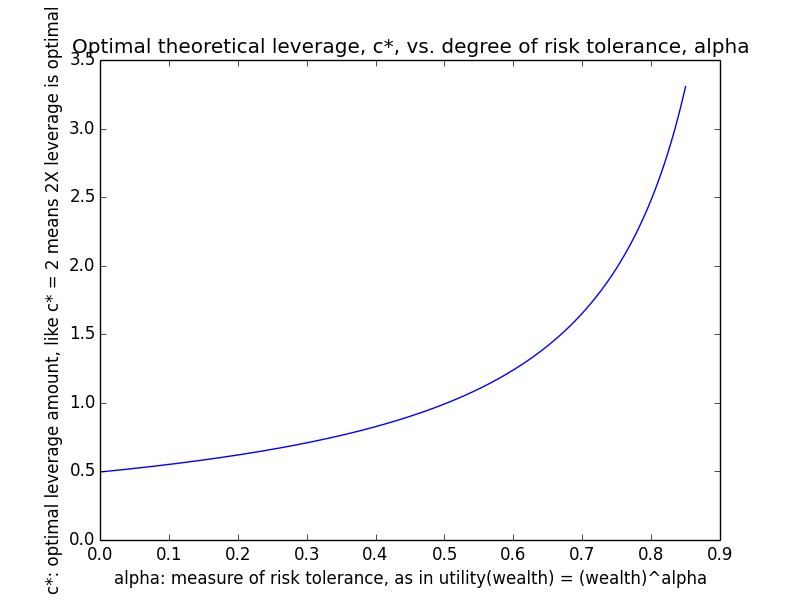
If we took a more optimistic value for μ (say, μ=0.08), we would instead have this graph:
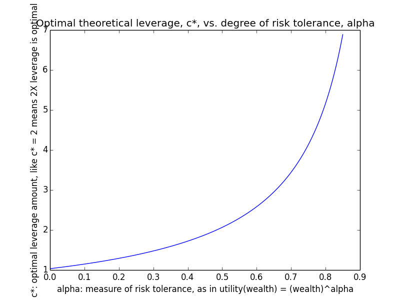
The equation c* = (μ-r) / [σ2(1-α)] works not just for α values between 0 and 1 but also (heuristically only!) for the edge cases: α = 0 and α = 1. If we say that α = 0 means utility(wealth) = ln(wealth), which is the assumption behind the Kelly criterion, then our equation falls back to the Kelly equation (Case 1). And for α = 1, utility(wealth) = wealth, so the investor is risk-neutral and thus should aim for infinite leverage (Case 2).
Simulations in the literature
"Leveraged Canadian Stock Portfolios: Long-Run Effects on Wealth and Risk" (2003) presents a simulation of leveraged investing based on actual historical returns between 1950 and 2001. The authors found that the optimal amount of leverage over this period would have been about 1.5X (rebalancing monthly). 4X leverage left almost no ending wealth, although this was partly because the simulation assumed monthly rebalancing, whereas daily rebalancing can reduce the risk of wipeout. The paper's Figure 1 shows an inverted U curve for the ending wealth of an investor from 1950 to 2001 as a function of how much leverage she used, between 1X and 4X. The paper's figure 2 shows that margin investing at 1.8X leverage was optimal in terms of median long-run performance, based on random monthly returns from 1950 to 2001 and assuming monthly rebalancing. (TODO: check that I got these details correct; reread study)
"Wealth and Risk from Leveraged Stock Portfolios" (2002) found optimal leverage of 1.7X assuming borrowing at 2% above Treasury bills. The authors note: "A modest amount of leverage enhances the performance of stock portfolios in the long run. However, higher amounts of leverage produce dramatic declines in long-run wealth."
My results
Case 1: Simplifying parameters in an attempt to match theory
Before getting simulation results for realistic parameter settings, I wanted to see how close I could get to the theoretical optimal-leverage results discussed above. Thus, I made many simplifying assumptions relative to the default configuration:
- no unemployment, inflation, taxes, or black swans
- invest a single lump sum at the beginning (the investor only earns one initial monthly paycheck on day 0)
- the investor doesn't ramp down leverage toward the end of the investing period
- the investor's voluntary leverage amount exactly equals the broker max rather than being set comfortably below the broker max, so that the investor maintains constant leverage.
While in the theoretical equations, the investor rebalances continuously, here the investor still rebalances only monthly (or daily when the broker liquidates securities to pay excessive margin).
The following graphj shows how well leverage does compared with non-leveraged investing as a function of the leverage amount. As in the tables above, I took utility(wealth) = √wealth. Each data point came from 1000 trials.
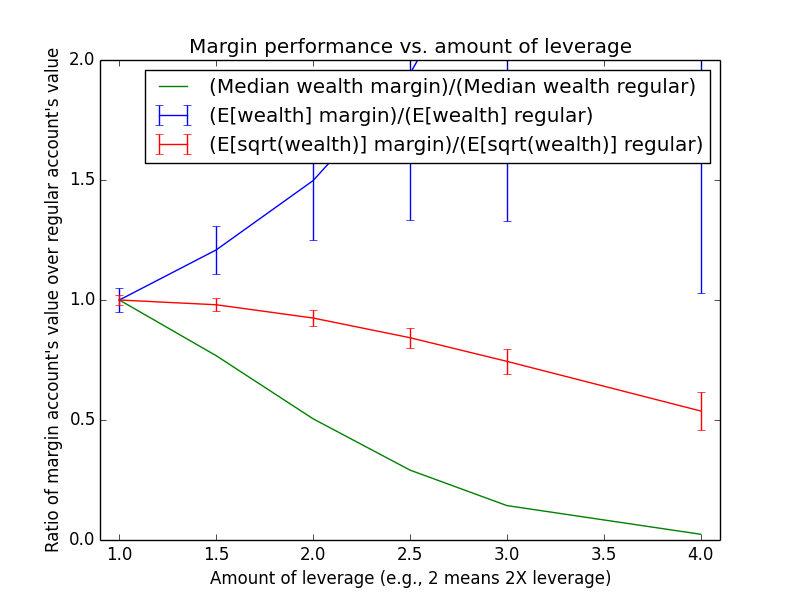
This graph agrees with the theory of optimal leverage discussed above. For α = 1 (expected utility is expected wealth), higher leverage keeps increasing expected utility. For α = 0.5 (expected utility is expected √wealth), theoretical optimal leverage is around ~1, which is what we see in the graph.
The sharp drop in the median with higher leverage underscores why commentators typically warn against constant-leverage investments like leveraged ETFs: Most of the time, the result is terrible, and it's only on rare occasions that you hit the jackpot.
How would the results change if, instead of investing a single lump sum at the beginning, the investor earned a monthly salary? As the Lifecycle Investing authors note, a regular salary is like a bond, so in some sense, investing salary each month should be less leveraged when the investor's whole lifetime assets. If the investor incurs huge losses early on, they can be compensated by later earnings. Following is the same graph as before except that the investor now earns a salary each month.
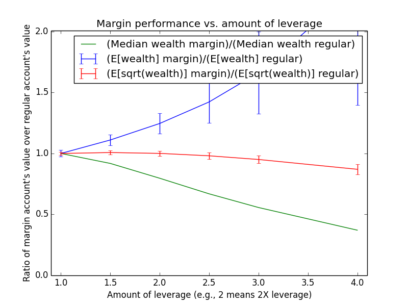
For high leverage amounts, the median performance is still worse than when not using leverage. One might think that the law of large numbers over many years would make leverage come out ahead, but this isn't the case because the 15-year performance of money initially invested in year 1 is correlated with the performance of money initially invested in year 2, and so on, since the whole amount of assets from previous years keeps getting invested in later years.
In theory, you could make results on successive years independent by investing the money earned in year n only during year n and then liquidating the investments. Over 15 independent years, this would tend to outperform investing without leverage the money earned in year n only during year n. But only investing for a year would miss out on returns from future years.
You could also invest the income earned in year n with leverage just in year n and then switch to non-leveraged investing for years n+1 and onwards. This also would probably outperform regular investing in the long run due to the law of large numbers(?), but the degree of outperformance would be small.
Case 2: Default (realistic) parameter values
The default margin configuration involves an investor earning income each month. The following graph shows optimal leverage with all parameters set at their default values. The huge gains and losses at higher leverage amounts that we saw in the previous two graphs are tempered because the default configuration tapers off leverage toward the end of the investing period (so, e.g., "4X leverage" isn't really 4X leverage for the whole period).
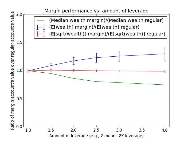
Different margin investing policies
No emergency savings
| Type | Mean ± stderr | Median | Min | Max | E[√wealth] ± stderr | σln(wealth) |
| Regular | $387,985 ± $7,688 | $328,643 | $73,896 | $2,612,862 | 599 ± 5 | 0.53 |
| Margin | $474,319 ± $25,047 | $270,926 | $11,255 | $16,106,461 | 604 ± 10 | 0.91 |
| Regular + 50% match | $581,977 ± $11,532 | $492,964 | $110,844 | $3,919,293 | 734 ± 7 | 0.53 |
Leverage is better than regular 33% of the time. Margin investor ended with no assets and a deficit in emergency savings 0.0% of the time. Leveraged account went fully bankrupt 0.0% of the time. Average simple-calculation margin ending balance was $462,480.
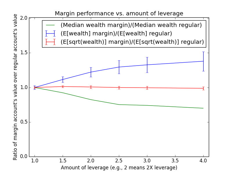


Emergency savings = $1 million
In this variant, emergency savings (invested without leverage) start at $1 million. This policy is also roughly what you'd get if you split between margin and non-margin investing with mostly non-margin investing. This variant can also approximate a policy where you donate a lot each year and only invest some money to donate at the end of the investing period because with that kind of policy, you move farther along the utility(wealth) curve before considering your donations of leveraged securities, just like if you donate appreciated emergency savings.
For example, suppose the first $1 million donated to a charity are crucial, while everything after that is less important. If you leverage most of your future donations, there's a risk you won't end with at least $1 million and so won't fill the crucial funding gap. In contrast, if you either have $1 million of emergency savings or donate a lot to the charity every year while working, then you'll probably donate at least the $1 million threshold, which means the further money that you're investing with leverage is less crucial and can be subjected to greater risk.
| Type | Mean ± stderr | Median | Min | Max | E[√wealth] ± stderr | σln(wealth) |
| Regular | $1,387,208 ± $44,538 | $1,008,288 | $78,803 | $23,424,760 | 1,088 ± 14 | 0.76 |
| Margin | $1,473,236 ± $60,853 | $962,294 | $78,572 | $36,980,834 | 1,090 ± 17 | 0.88 |
| Regular + 50% match | $1,581,200 ± $47,967 | $1,170,909 | $118,204 | $24,731,191 | 1,169 ± 15 | 0.73 |
Leverage is better than regular 34% of the time. Margin investor ended with no assets and a deficit in emergency savings 0.0% of the time. Leveraged account went fully bankrupt 0.0% of the time. Average simple-calculation margin ending balance was $1,461,627.
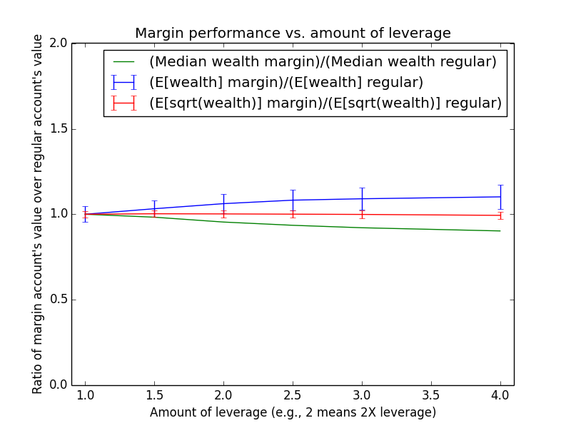
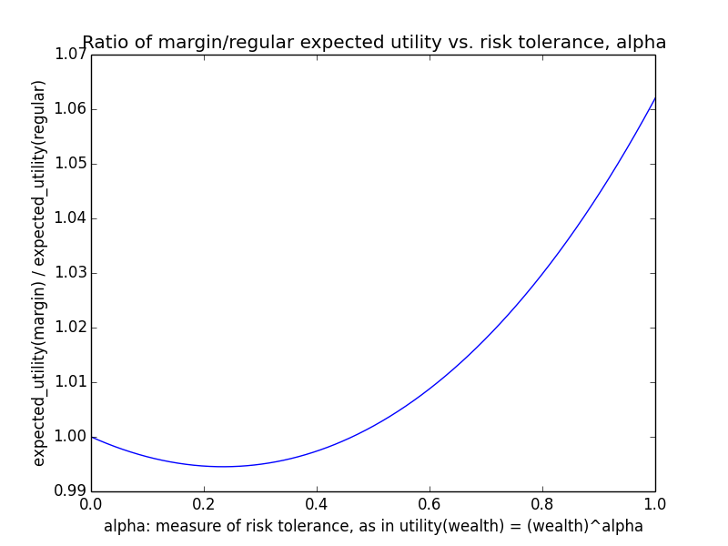
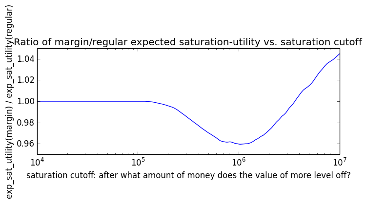
Don't taper off leverage near end of investing period
| Type | Mean ± stderr | Median | Min | Max | E[√wealth] ± stderr | σln(wealth) |
| Regular | $487,907 ± $11,052 | $395,493 | $78,803 | $4,694,052 | 667 ± 7 | 0.58 |
| Margin | $574,030 ± $28,395 | $341,607 | $27,854 | $18,215,480 | 670 ± 11 | 0.88 |
| Regular + 50% match | $681,900 ± $14,845 | $558,923 | $118,204 | $6,000,483 | 790 ± 8 | 0.57 |
Leverage is better than regular 33% of the time. Margin investor ended with no assets and a deficit in emergency savings 0.0% of the time. Leveraged account went fully bankrupt 0.0% of the time. Average simple-calculation margin ending balance was $562,226.
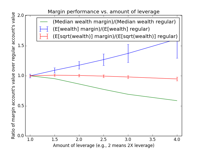
The optimal-leverage graph above shows that when we don't taper off higher leverage amounts toward the end of the simulation period, the expected-value curve is able to be concave up instead of concave down the way it normally is. Of course, the median also shoots down more dramatically than usual.
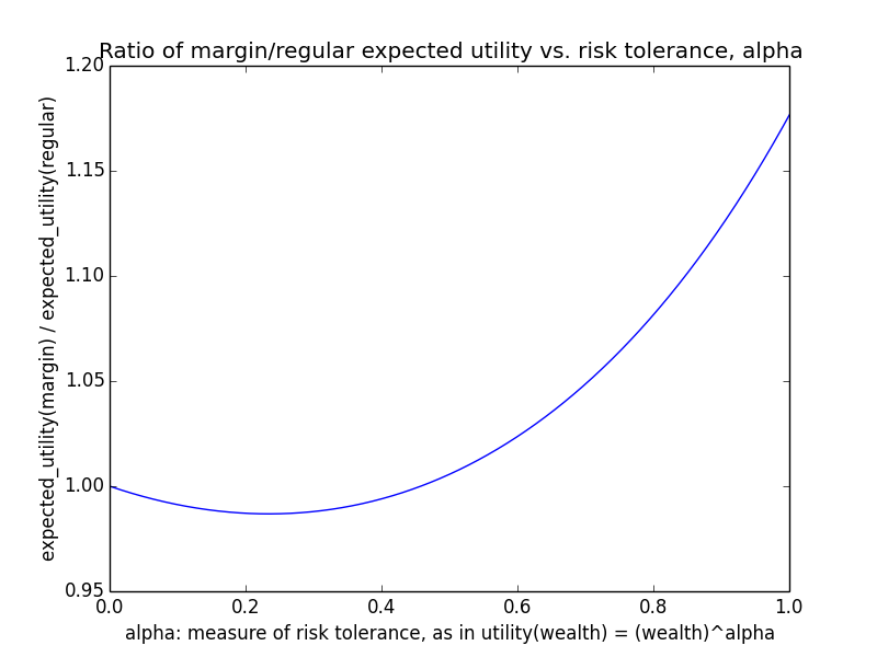

Taper off leverage a lot near end of investing period
In this variant, the investor decreases leverage aggressively toward the end of the investing period. In particular, the max leverage Y years before the end can be at most 1 + 0.1Y. For instance, 5 years before the end, the max leverage can be at most 1.5X. The purpose of running this variant was to see if I could get closer to the results presented in Lifecycle Investing in which early leverage followed by dramatic tapering down in later years allows for better median outcomes than unleveraged investing. My leverage ramp-down here is only approximate and isn't based on exactly targeting a constant proportion of lifetime wealth toward equity. Moreover, I haven't implemented fixed-income investing into my simulation, so my leveraged investors always have more total equity-years of exposure than unleveraged. Probably for this reason, I still found that leverage reduces median outcomes. I hope that if I were to allow investors in the simulation to buy fixed-income securities that I could reproduce the Lifecycle Investing results (otherwise I'd worry about a bug in my code), but I haven't done that due to lack of time.
| Type | Mean ± stderr | Median | Min | Max | E[√wealth] ± stderr | σln(wealth) |
| Regular | $487,907 ± $11,052 | $395,493 | $78,803 | $4,694,052 | 667 ± 7 | 0.58 |
| Margin | $532,346 ± $18,001 | $381,385 | $71,896 | $10,155,955 | 676 ± 9 | 0.71 |
| Regular + 50% match | $681,900 ± $14,845 | $558,923 | $118,204 | $6,000,483 | 790 ± 8 | 0.57 |
Leverage is better than regular 34% of the time. Margin investor ended with no assets and a deficit in emergency savings 0.0% of the time. Leveraged account went fully bankrupt 0.0% of the time. Average simple-calculation margin ending balance was $521,464.
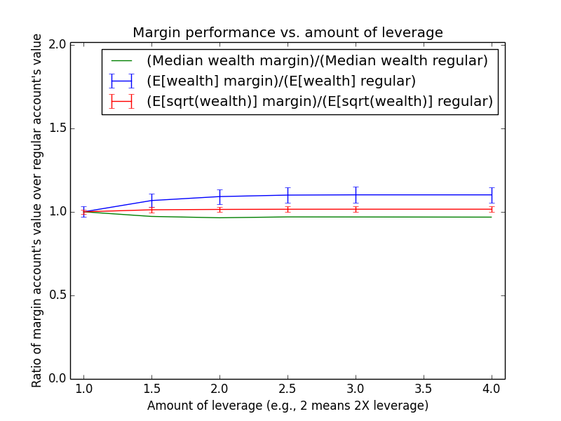
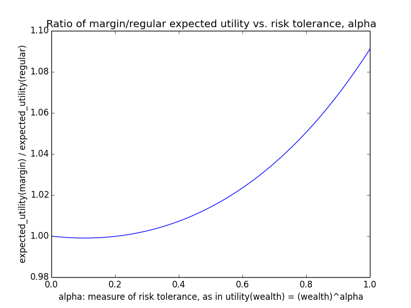
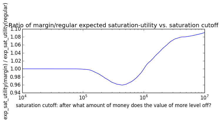
Don't rebalance monthly
In this configuration, the investor buys new shares at the standard leverage ratio but doesn't rebalance existing shares to increase leverage when asset prices rise. This tends to cause margin-to-assets ratios to fall over time as asset values appreciate without corresponding increases in debt.
I think this approach is somewhat similar to the constant-debt strategy discussed later, in the sense that for any given paycheck, that paycheck is invested with some initial amount of debt, and that debt isn't increased as asset prices rise. That said, my simulated investor may not be able to maintain constant debt when asset prices fall because the simulation assumes that the investor's leverage starts out close to the maximum leverage allowed by the broker, which may not be true in the real world. So these simulations shouldn't be taken as an indication of how a true constant-debt strategy would perform.
| Type | Mean ± stderr | Median | Min | Max | E[√wealth] ± stderr | σln(wealth) |
| Regular | $487,907 ± $11,052 | $395,493 | $78,803 | $4,694,052 | 667 ± 7 | 0.58 |
| Margin | $523,641 ± $15,173 | $388,554 | $32,437 | $6,292,376 | 671 ± 9 | 0.78 |
| Regular + 50% match | $681,900 ± $14,845 | $558,923 | $118,204 | $6,000,483 | 790 ± 8 | 0.57 |
Leverage is better than regular 46% of the time. Margin investor ended with no assets and a deficit in emergency savings 0.0% of the time. Leveraged account went fully bankrupt 0.0% of the time. Average simple-calculation margin ending balance was $519,847.
The margin median here is much higher than usual, but the upside of margin is much smaller. Maybe this variant is what people have in mind when they say that margin investing is less risky than constant-leverage leveraged ETFs.
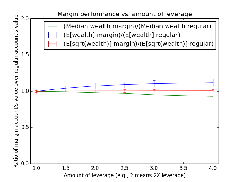
Remember that "2.5X leverage" isn't really 2.5X because in this setting, the investor only rebalances when asset prices fall, not when they rise, so the investor is actually not fully leveraged much of the time.


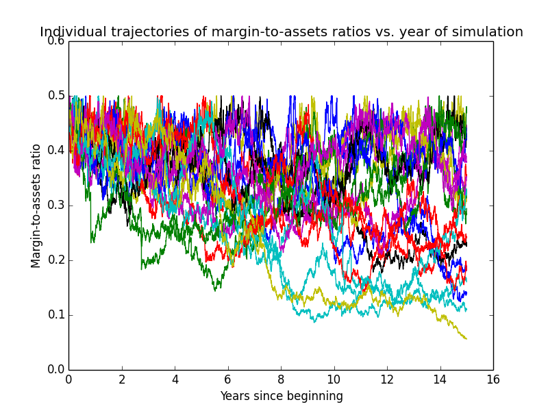
There are many fewer accumulated capital losses than in the default configuration because if leverage is less than 2X, there's much less selling of securities to meet margin requirements:
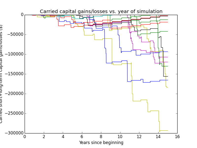
This variant still does annual tax-loss harvesting, but apparently the losses accumulated from yearly harvesting are much smaller than those that can be harvested when rebalancing in response to losses on a daily basis (which the default simulation does more than this version).
Don't rebalance monthly and don't taper off leverage toward end
| Type | Mean ± stderr | Median | Min | Max | E[√wealth] ± stderr | σln(wealth) |
| Regular | $487,907 ± $11,052 | $395,493 | $78,803 | $4,694,052 | 667 ± 7 | 0.58 |
| Margin | $523,675 ± $15,175 | $388,625 | $32,437 | $6,292,376 | 671 ± 9 | 0.78 |
| Regular + 50% match | $681,900 ± $14,845 | $558,923 | $118,204 | $6,000,483 | 790 ± 8 | 0.57 |
Leverage is better than regular 46% of the time. Margin investor ended with no assets and a deficit in emergency savings 0.0% of the time. Leveraged account went fully bankrupt 0.0% of the time. Average simple-calculation margin ending balance was $519,848.
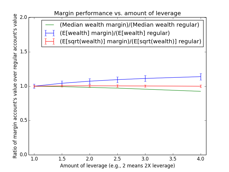
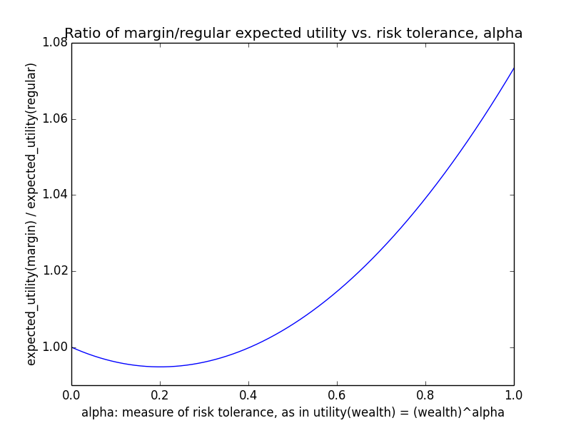
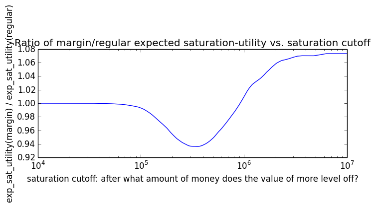
Don't rebalance monthly and pay principal throughout
This is the most conservative strategy. Leverage can be made less risky if, instead of keeping your loans around until the end of the investing period, you pay them off over time as if you were paying off a home mortgage. Doing this means you're less leveraged at later times, as this graph shows (for the 2X leverage configuration):
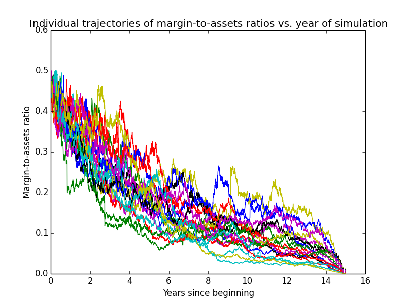
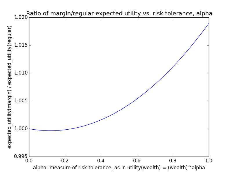
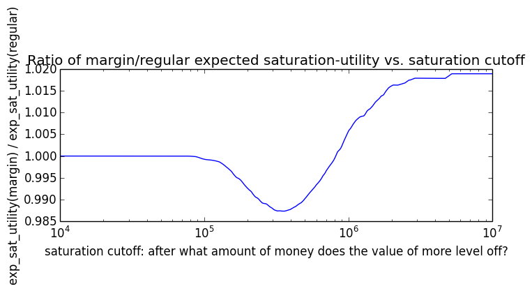
Obviously this configuration is incompatible with the default policy of rebalancing back up to 2X leverage, since paying off principal throughout reduces the margin-to-assets ratio over time, while a policy of rebalancing to increase leverage would undo that.
For this variation, I used a regular annuity mortgage calculation to pay off principal such that the investor's margin loans would be fully paid off on the exact date when the investor donates the securities.k (If the investor doesn't have enough income one month to pay off principal, she sells some of her investments to pay for it. In the simulations I've run, this only happens during months when she's laid off.)
We can see from the results table for this method that it's more certain to outperform non-margin investing due to its safety, though it also has less of an edge over non-margin investing.
| Type | Mean ± stderr | Median | Min | Max | E[√wealth] ± stderr | σln(wealth) |
| Regular | $487,907 ± $11,052 | $395,493 | $78,803 | $4,694,052 | 667 ± 7 | 0.58 |
| Margin | $497,137 ± $12,075 | $395,383 | $76,191 | $5,224,349 | 669 ± 7 | 0.62 |
| Regular + 50% match | $681,900 ± $14,845 | $558,923 | $118,204 | $6,000,483 | 790 ± 8 | 0.57 |
Leverage is better than regular 48% of the time. Margin investor ended with no assets and a deficit in emergency savings 0.0% of the time. Leveraged account went fully bankrupt 0.0% of the time. Average simple-calculation margin ending balance was $496,471.
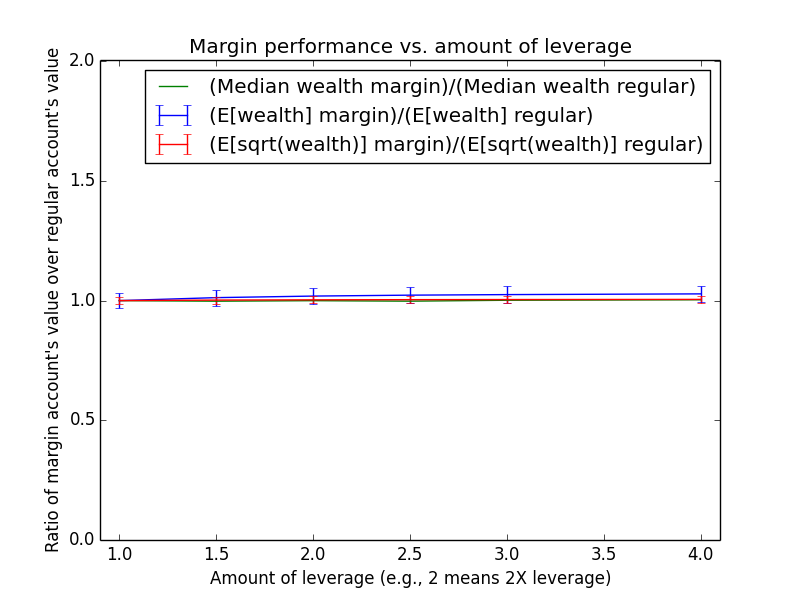
Discussion
The summary of these graphs is what one would have expected: Policies that keep you more leveraged for longer have higher expected value but also lower median value.
Parameter sensitivity analysis
This section explores how the results change with different parameter configurations, to help ensure that the findings are not specific to the particular input assumptions I made.
Assume that Interactive Brokers margin liquidations sell the most tax-advantaged lots first
In the default simulation, I assumed that if you exceed your broker's margin threshold, your broker sells securities randomly to pay off debts, without consideration of whether securities will incur positive capital-gains taxes. This variant instead assumes that your broker liquidates the securities with the biggest percent losses first.
| Type | Mean ± stderr | Median | Min | Max | E[√wealth] ± stderr | σln(wealth) |
| Regular | $487,907 ± $11,052 | $395,493 | $78,803 | $4,694,052 | 667 ± 7 | 0.58 |
| Margin | $574,184 ± $28,426 | $341,617 | $27,864 | $18,265,230 | 671 ± 11 | 0.88 |
| Regular + 50% match | $681,900 ± $14,845 | $558,923 | $118,204 | $6,000,483 | 790 ± 8 | 0.57 |
Leverage is better than regular 33% of the time. Margin investor ended with no assets and a deficit in emergency savings 0.0% of the time. Leveraged account went fully bankrupt 0.0% of the time. Average simple-calculation margin ending balance was $562,226.
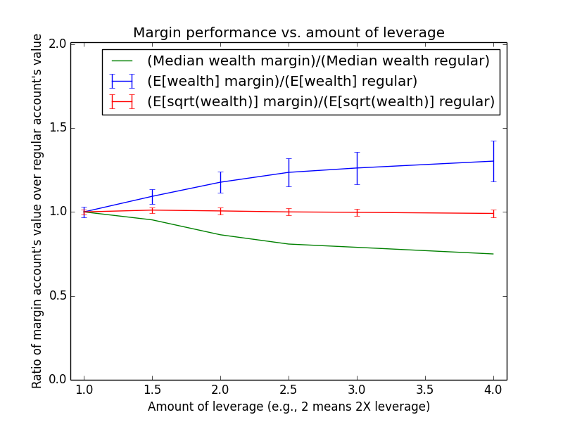


Here are some accumulated capital losses for the 2X-leverage version of this configuration:
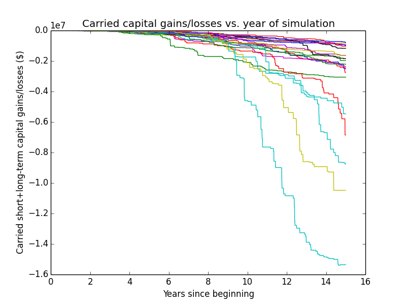
What is IB's actual liquidation algorithm?
IB says: "IB employs a proprietary algorithm which identifies positions for liquidation. This is a complicated formula which seeks always to make the best possible liquidation. There are numerous factors involved in the liquidation algorithm which are taken into account prior to the creation of a liquidation trade." One forum reports about IB: "if you are -1 or -2 in your margin they will liquidate 100 contracts regardless from ANY position, whichever pleases them", with the aim of maximizing IB's profit.
IB explains that IB allows you to set a position that you prefer to be liquidated last: "This feature allows you to mark those positions which you would prefer to hold over others. IB will try to honor those requests, but this is merely a request and we cannot guarantee that the chosen position won’t be liquidated." I don't know if you can select a bunch of positions to liquidate last or just one.
In any case, the liquidation order didn't seem to make a big difference to my simulation results, presumably because most liquidations happen when there are huge market losses, which means many individual securities have losses.
Use VIX daily volatilities
The default simulation assumes a constant annualized volatility of σ = 0.22. In the real world, volatility swings a lot and sometimes reaches very high levels. How much does this affect the results? To see, I downloaded VIX data from CBOE between 2004 and 2015. This gave a list of volatility numbers. In the simulation, I let the daily volatility values run through that list in order, and if the simulation had more days than the VIX data, I cycled through from the start again. The VIX data include the crash of 2008 (see here for a chart of the data), so probably this data set overstates volatility relative to typical market conditions.
| Type | Mean ± stderr | Median | Min | Max | E[√wealth] ± stderr | σln(wealth) |
| Regular | $484,101 ± $10,897 | $394,473 | $90,550 | $4,092,341 | 664 ± 7 | 0.58 |
| Margin | $565,603 ± $26,965 | $334,188 | $40,135 | $14,978,160 | 667 ± 11 | 0.87 |
| Regular + 50% match | $677,110 ± $14,693 | $554,650 | $131,440 | $5,225,361 | 788 ± 8 | 0.56 |
Leverage is better than regular 31% of the time. Margin investor ended with no assets and a deficit in emergency savings 0.0% of the time. Leveraged account went fully bankrupt 0.0% of the time. Average simple-calculation margin ending balance was $554,769.
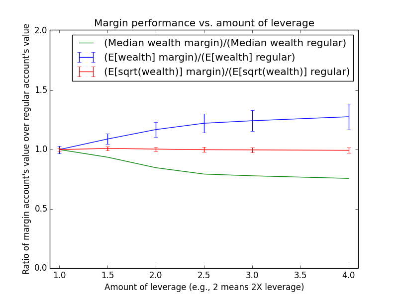
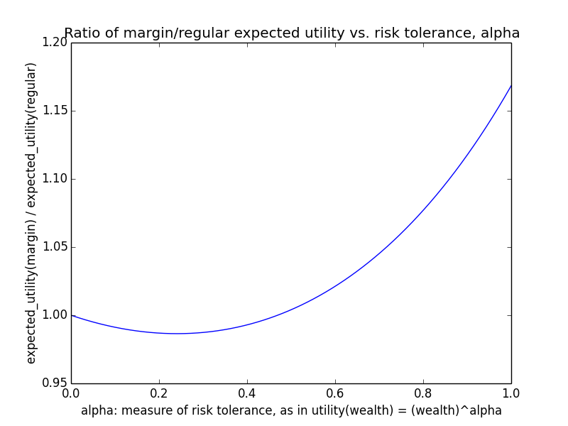
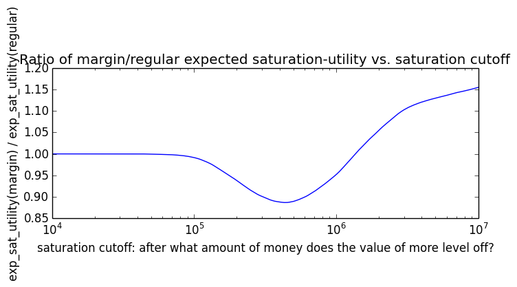
Invest for 5 years instead of 15
| Type | Mean ± stderr | Median | Min | Max | E[√wealth] ± stderr | σln(wealth) |
| Regular | $235,659 ± $3,067 | $215,625 | $68,288 | $651,283 | 476 ± 3 | 0.40 |
| Margin | $244,873 ± $4,401 | $208,466 | $0 | $982,008 | 477 ± 4 | 0.66 |
| Regular + 50% match | $303,668 ± $3,757 | $280,627 | $92,932 | $806,853 | 541 ± 3 | 0.38 |
Leverage is better than regular 39% of the time. Margin investor ended with no assets and a deficit in emergency savings 0.1% of the time. Leveraged account went fully bankrupt 0.1% of the time. Average simple-calculation margin ending balance was $241,507.
A main reason why these numbers aren't as low as one might think compared with 15-year results is that both 5-year and 15 results have the same initial emergency savings of $100,000 added to their totals.
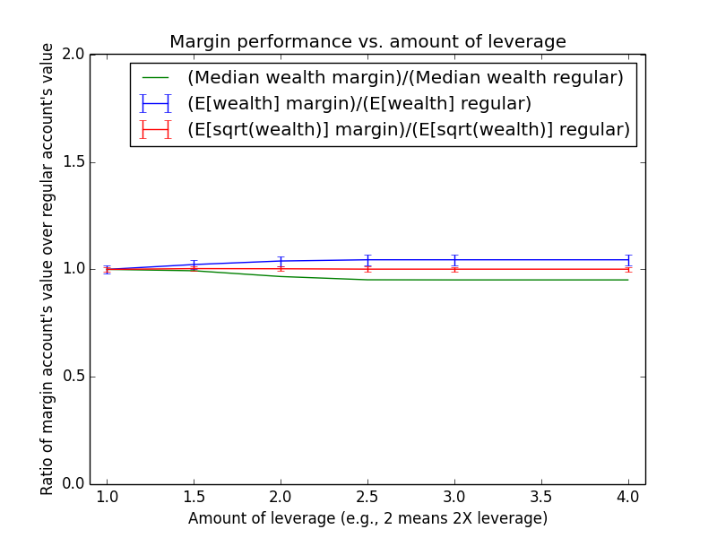
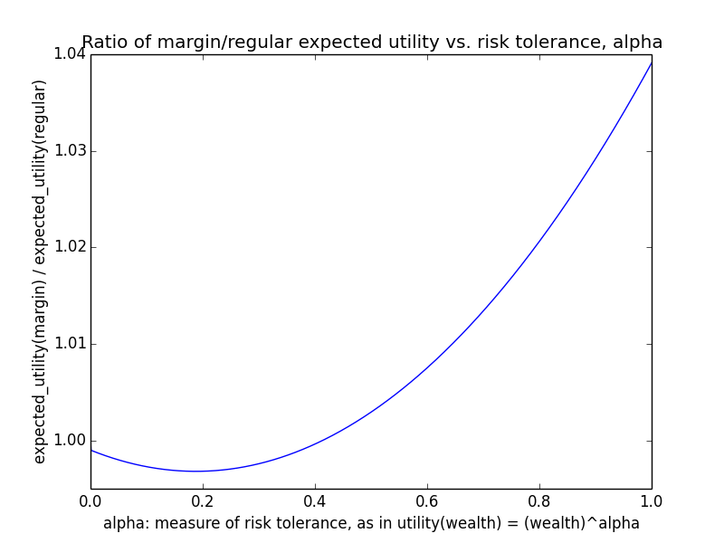
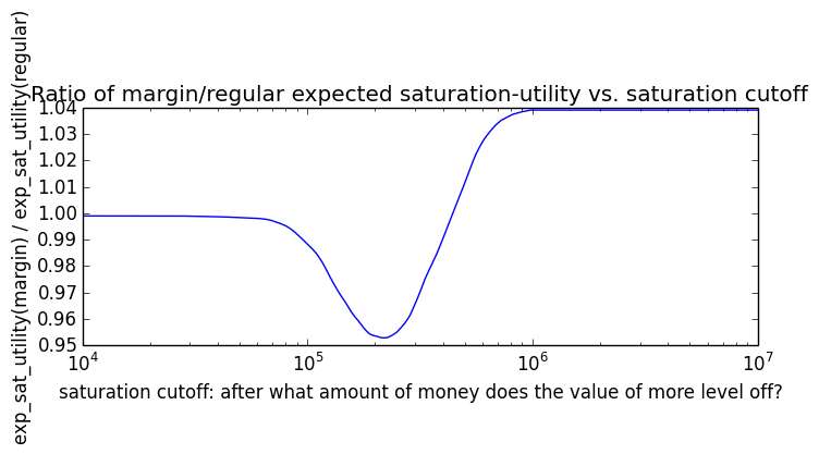
Invest for 30 years instead of 15
| Type | Mean ± stderr | Median | Min | Max | E[√wealth] ± stderr | σln(wealth) |
| Regular | $790,905 ± $26,320 | $537,613 | $81,225 | $8,536,976 | 817 ± 11 | 0.76 |
| Margin | $1,045,368 ± $83,950 | $382,313 | $27,784 | $37,624,878 | 803 ± 20 | 1.16 |
| Regular + 50% match | $1,139,063 ± $37,027 | $783,143 | $121,191 | $11,490,872 | 983 ± 13 | 0.75 |
Leverage is better than regular 21% of the time. Margin investor ended with no assets and a deficit in emergency savings 0.0% of the time. Leveraged account went fully bankrupt 0.0% of the time. Average simple-calculation margin ending balance was $1,016,700.
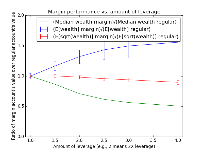
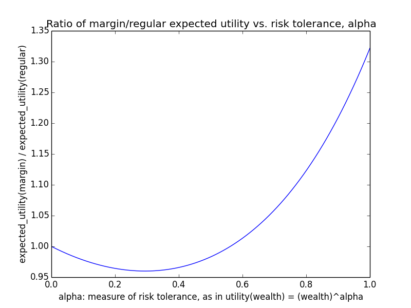
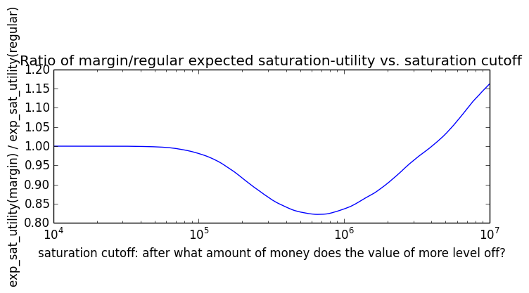
Unemployment lasts a long time
This variant sets the monthly probability of unemployment to 4% and the monthly probability of becoming employed during a period of unemployment also to 4%. In other words, the investor becomes unemployed roughly every ~2 years on average, and this lasts for ~2 years on average. This can help approximate the income profile for a serial entrepreneur who doesn't earn much during the first 2 years of founding her company.
I added this variant after computing the rest of this essay and so copy-pasted these results in manually. The following results are as of 30 May 2015 and might possibly not be up to date by the time you read this.
| Type | Mean ± stderr | Median | Min | Max | E[√wealth] ± stderr | σln(wealth) |
| Regular | $305,120 ± $7,789 | $243,060 | $16,943 | $2,991,945 | 521 ± 6 | 0.68 |
| Margin | $353,700 ± $16,931 | $214,078 | $13,620 | $8,282,302 | 525 ± 9 | 0.93 |
| Regular + 50% match | $407,719 ± $10,018 | $331,967 | $25,415 | $3,447,322 | 604 ± 7 | 0.67 |
Leverage is better than regular 29% of the time. Margin investor ended with no assets and a deficit in emergency savings 0.0% of the time. Leveraged account went fully bankrupt 0.0% of the time. Average simple-calculation margin ending balance was $342,404.
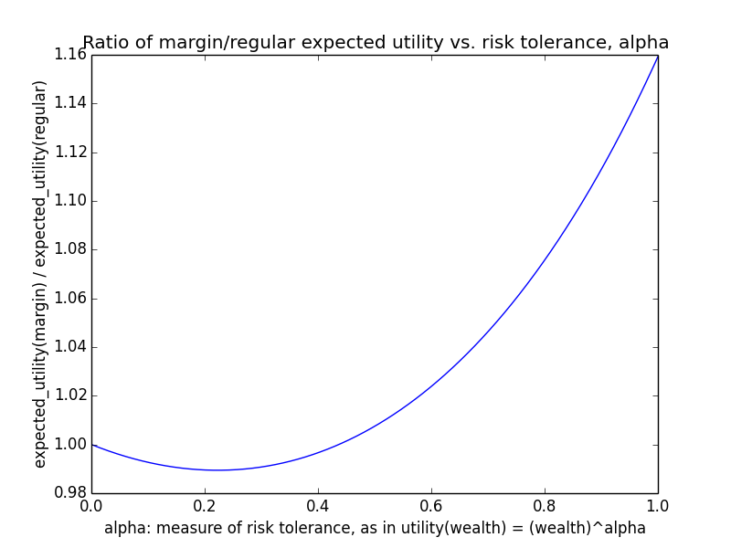
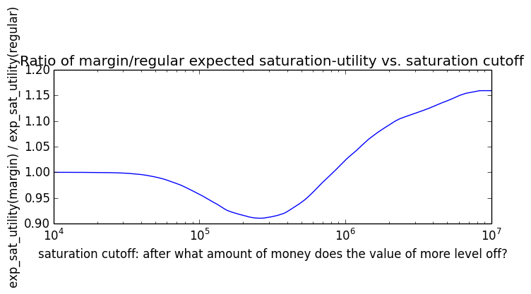
The absolute wealth numbers are lower for both regular and margin investing because of longer periods of unemployment, but the comparison between regular vs. margin investing looks very similar as it did when using default settings.
μ = 0.1
| Type | Mean ± stderr | Median | Min | Max | E[√wealth] ± stderr | σln(wealth) |
| Regular | $382,489 ± $9,577 | $301,462 | $43,798 | $4,287,350 | 585 ± 6 | 0.63 |
| Margin | $596,718 ± $35,674 | $313,378 | $22,834 | $24,959,801 | 663 ± 13 | 0.99 |
| Regular + 50% match | $523,922 ± $12,593 | $417,278 | $65,697 | $5,393,793 | 687 ± 7 | 0.62 |
Leverage is better than regular 54% of the time. Margin investor ended with no assets and a deficit in emergency savings 0.0% of the time. Leveraged account went fully bankrupt 0.0% of the time. Average simple-calculation margin ending balance was $586,080.
The ending-wealth values are lower than you might expect because I'm discounting by exp(-μt), so a higher μ implies more discounting. The undiscounted values should be higher than for other variants because of higher μ.
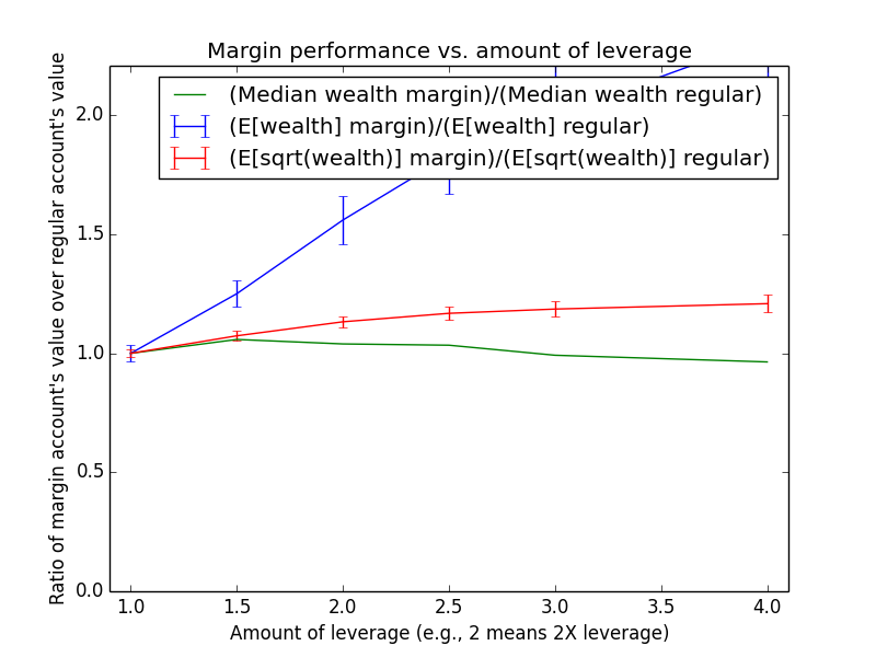
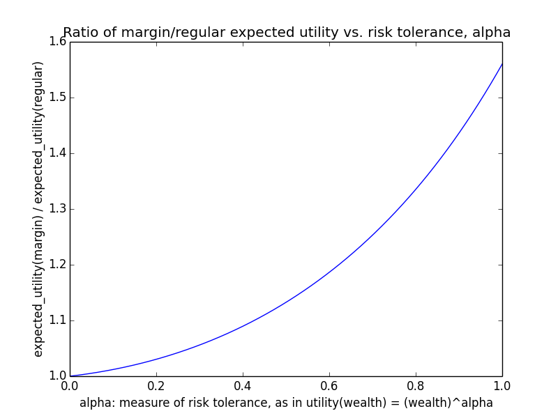
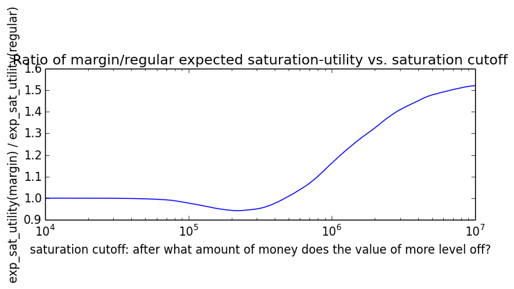
μ = 0.1 and don't rebalance monthly
| Type | Mean ± stderr | Median | Min | Max | E[√wealth] ± stderr | σln(wealth) |
| Regular | $382,489 ± $9,577 | $301,462 | $43,798 | $4,287,350 | 585 ± 6 | 0.63 |
| Margin | $450,527 ± $13,275 | $336,909 | $27,274 | $5,733,803 | 621 ± 8 | 0.79 |
| Regular + 50% match | $523,922 ± $12,593 | $417,278 | $65,697 | $5,393,793 | 687 ± 7 | 0.62 |
Leverage is better than regular 70% of the time. Margin investor ended with no assets and a deficit in emergency savings 0.0% of the time. Leveraged account went fully bankrupt 0.0% of the time. Average simple-calculation margin ending balance was $449,163.
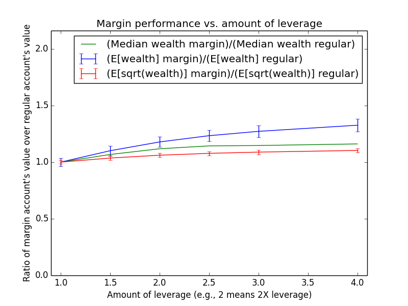
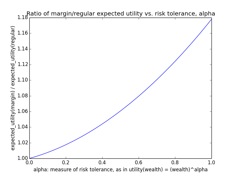
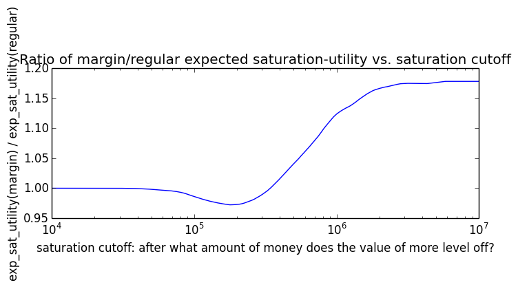
μ = 0.07
| Type | Mean ± stderr | Median | Min | Max | E[√wealth] ± stderr | σln(wealth) |
| Regular | $445,881 ± $10,477 | $358,323 | $64,209 | $4,538,824 | 635 ± 6 | 0.60 |
| Margin | $575,228 ± $30,478 | $328,815 | $25,703 | $20,202,492 | 664 ± 12 | 0.92 |
| Regular + 50% match | $618,912 ± $13,967 | $501,799 | $96,313 | $5,768,797 | 751 ± 7 | 0.58 |
Leverage is better than regular 40% of the time. Margin investor ended with no assets and a deficit in emergency savings 0.0% of the time. Leveraged account went fully bankrupt 0.0% of the time. Average simple-calculation margin ending balance was $563,819.
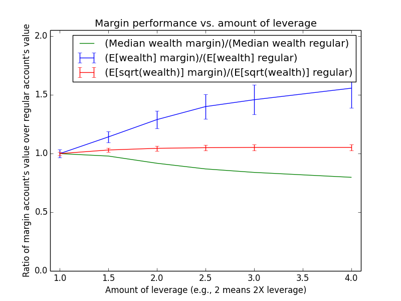
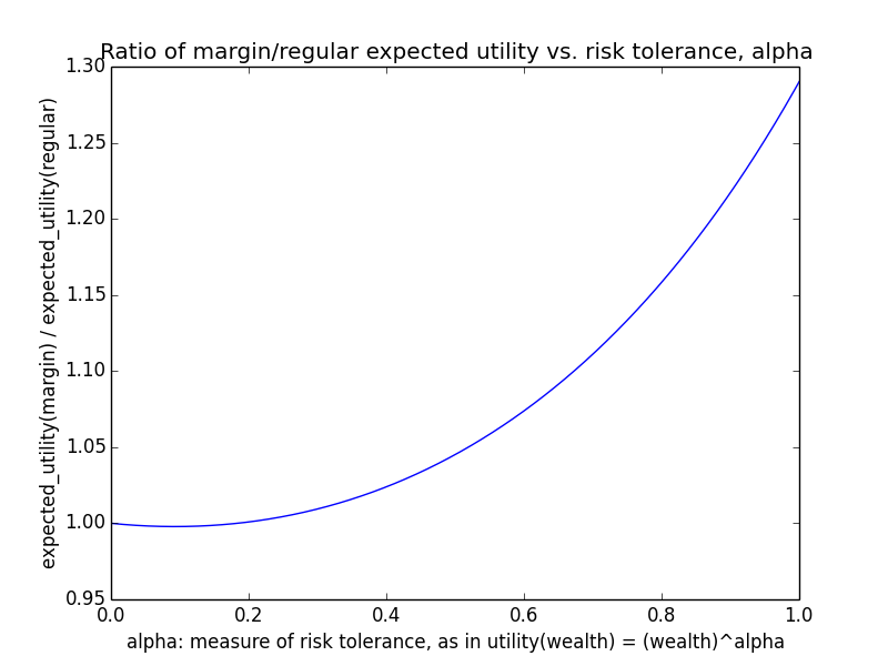
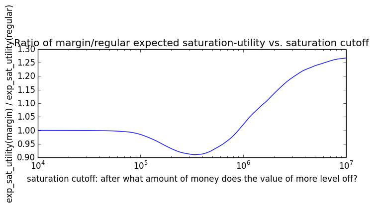
μ = 0.04
| Type | Mean ± stderr | Median | Min | Max | E[√wealth] ± stderr | σln(wealth) |
| Regular | $530,510 ± $11,622 | $436,065 | $94,312 | $4,844,166 | 697 ± 7 | 0.57 |
| Margin | $578,941 ± $26,906 | $353,887 | $30,195 | $16,726,627 | 679 ± 11 | 0.85 |
| Regular + 50% match | $745,760 ± $15,714 | $617,249 | $139,465 | $6,224,654 | 828 ± 8 | 0.55 |
Leverage is better than regular 24% of the time. Margin investor ended with no assets and a deficit in emergency savings 0.0% of the time. Leveraged account went fully bankrupt 0.0% of the time. Average simple-calculation margin ending balance was $566,786.
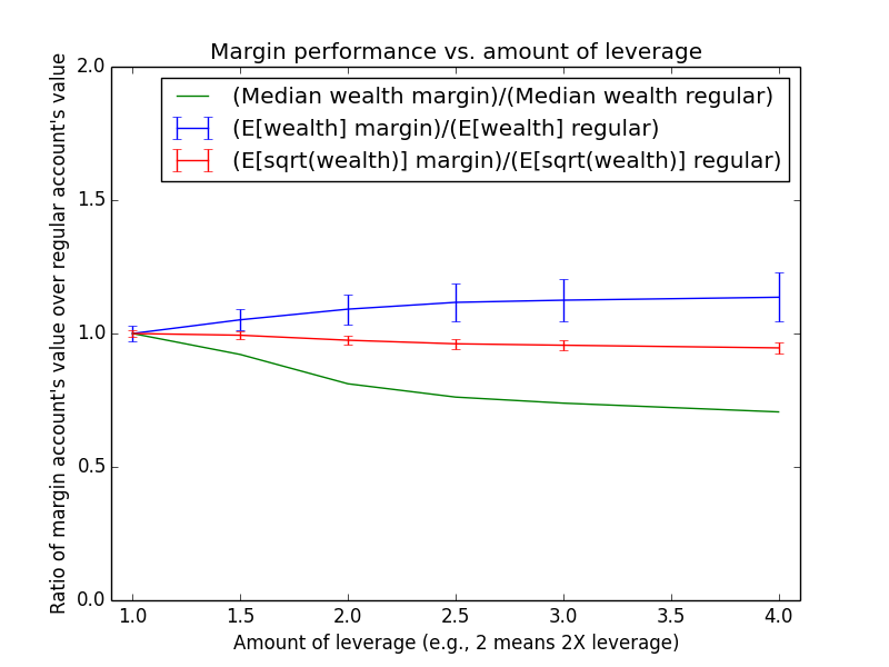
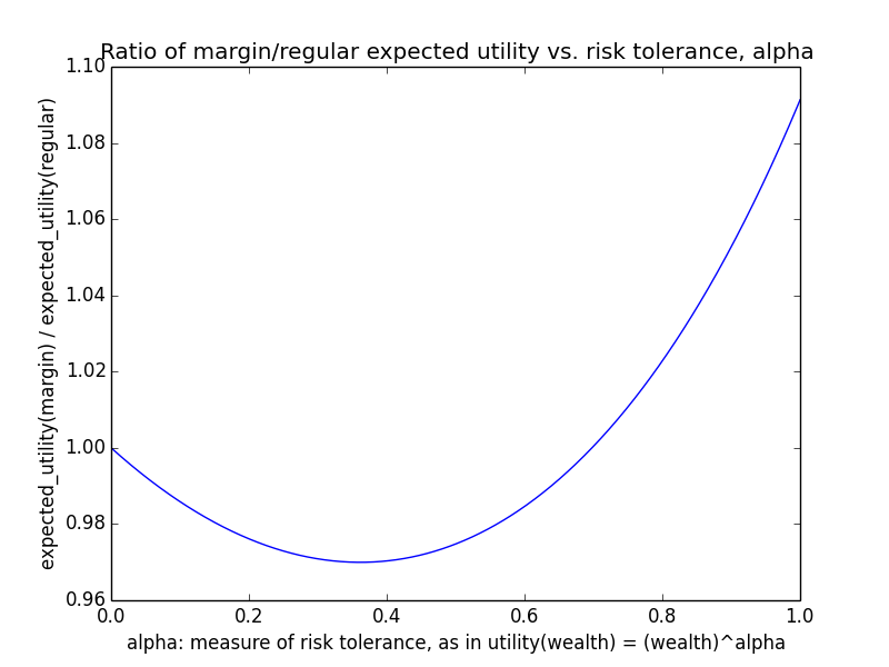
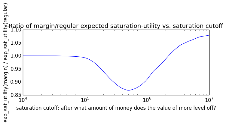
μ = -0.02
| Type | Mean ± stderr | Median | Min | Max | E[√wealth] ± stderr | σln(wealth) |
| Regular | $800,927 ± $15,034 | $683,108 | $170,863 | $5,687,094 | 865 ± 7 | 0.50 |
| Margin | $671,775 ± $23,462 | $477,772 | $47,230 | $12,190,740 | 757 ± 10 | 0.73 |
| Regular + 50% match | $1,151,203 ± $20,915 | $989,213 | $250,059 | $7,484,889 | 1,039 ± 9 | 0.49 |
Leverage is better than regular 7% of the time. Margin investor ended with no assets and a deficit in emergency savings 0.0% of the time. Leveraged account went fully bankrupt 0.0% of the time. Average simple-calculation margin ending balance was $657,397.
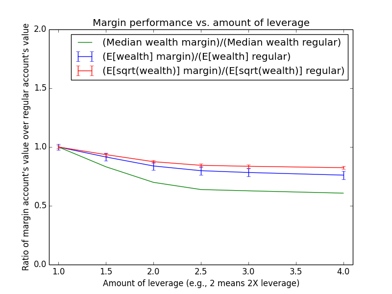
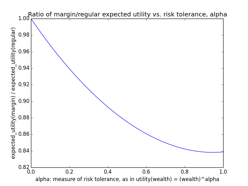
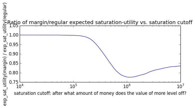
σ = 0.40
| Type | Mean ± stderr | Median | Min | Max | E[√wealth] ± stderr | σln(wealth) |
| Regular | $498,963 ± $32,517 | $275,959 | $37,239 | $25,964,368 | 614 ± 11 | 0.91 |
| Margin | $658,190 ± $153,283 | $171,210 | $11,546 | $145,717,959 | 557 ± 19 | 1.24 |
| Regular + 50% match | $696,238 ± $41,870 | $397,180 | $55,314 | $32,222,930 | 732 ± 13 | 0.89 |
Leverage is better than regular 9% of the time. Margin investor ended with no assets and a deficit in emergency savings 0.0% of the time. Leveraged account went fully bankrupt 0.0% of the time. Average simple-calculation margin ending balance was $634,085.
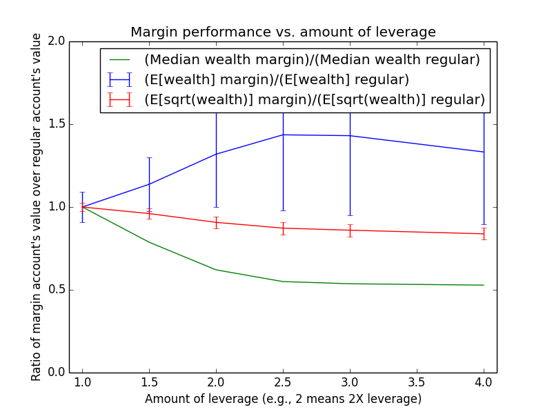
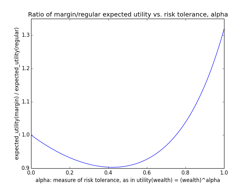
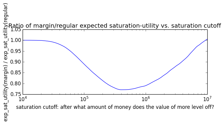
σ = 0, no black swans, no unemployment
This variant is mainly useful for debugging. It helps show what effect stock-market and unemployment randomness have on the results.
| Type | Mean ± stderr | Median | Min | Max | E[√wealth] ± stderr | σln(wealth) |
| Regular | $525,316 ± $0 | $525,316 | $525,316 | $525,316 | 725 ± 0 | 0.00 |
| Margin | $584,555 ± $0 | $584,555 | $584,555 | $584,555 | 765 ± 0 | 0.00 |
| Regular + 50% match | $737,978 ± $0 | $737,978 | $737,978 | $737,978 | 859 ± 0 | 0.00 |
Leverage is better than regular 100% of the time. Margin investor ended with no assets and a deficit in emergency savings 0.0% of the time. Leveraged account went fully bankrupt 0.0% of the time. Average simple-calculation margin ending balance was $595,555.
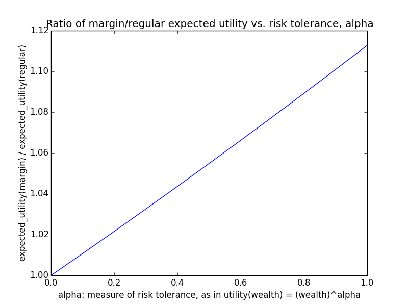
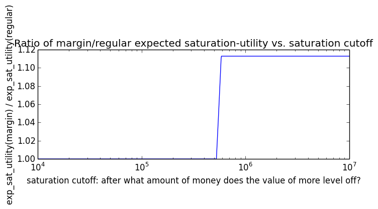
Margin interest rate = 1.5%
The actual margin interest rate for Interactive Brokers in 2015 is around 1.5%, so I wanted to test this parameter setting rather than just the default, more cautious value of 3.0%. With μ = 5.4%, this implies an equity premium of ~4%.
| Type | Mean ± stderr | Median | Min | Max | E[√wealth] ± stderr | σln(wealth) |
| Regular | $487,907 ± $11,052 | $395,493 | $78,803 | $4,694,052 | 667 ± 7 | 0.58 |
| Margin | $622,548 ± $31,826 | $364,678 | $28,414 | $20,695,065 | 695 ± 12 | 0.90 |
| Regular + 50% match | $681,900 ± $14,845 | $558,923 | $118,204 | $6,000,483 | 790 ± 8 | 0.57 |
Leverage is better than regular 38% of the time. Margin investor ended with no assets and a deficit in emergency savings 0.0% of the time. Leveraged account went fully bankrupt 0.0% of the time. Average simple-calculation margin ending balance was $611,502.
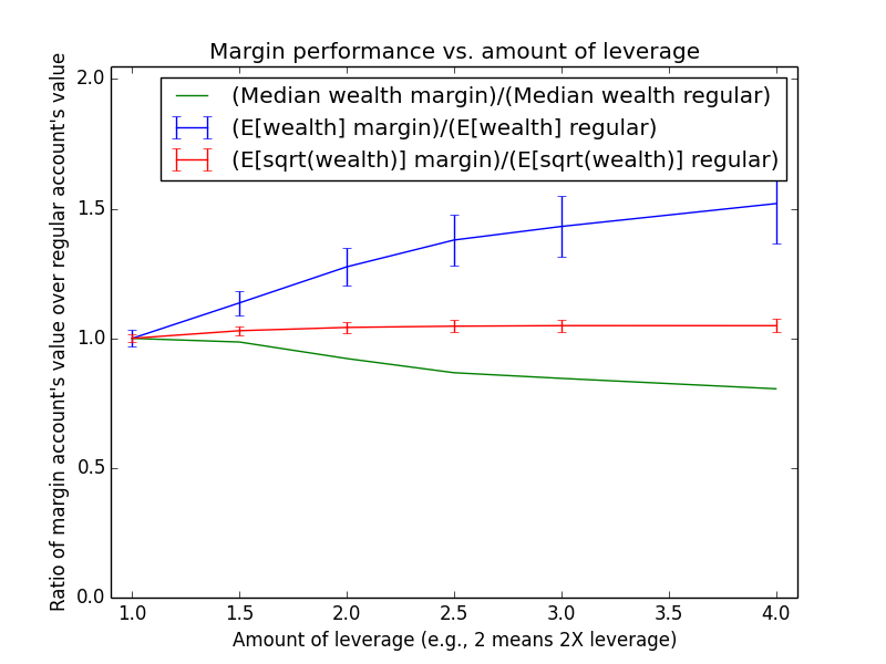
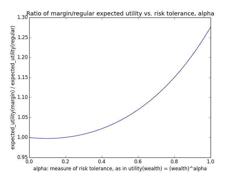
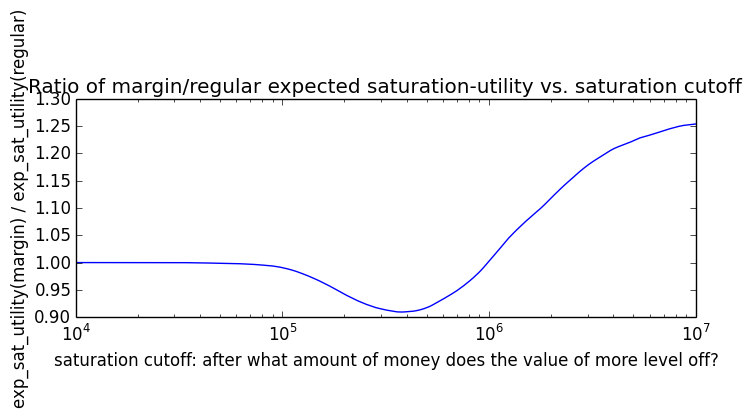
Further simulation features that could be implemented
Strategies to dynamically vary leverage
Lifecycle Investing (ch. 4) proposes two ways to adjust leverage over time to potentially improve risk-adjusted performance:
- Reduce leverage when CAPE is higher because this suggests possibly a lower future μ
- Reduce leverage when future volatility forecasts (e.g., VIX) are higher because this implies higher σ.
Both of these seem like reasonable approaches if
- you have enough time to actively make these changes
- you're trading in a tax-advantaged account (e.g., IRA).
Adjusting leverage downward in a taxable account would mean selling shares and incurring capital-gains taxes, unless you pay down debt using new income rather than already invested assets.
Two other obvious reasons to adjust leverage based on the optimal-leverage formulas discussed previously would be
- if the borrowing interest rate r changes or
- if your risk tolerance α changes (depending on how sharply it looks like your future donations would hit diminishing marginal returns).
Using actual daily returns
In my simulations, I assumed normally distributed daily returns with black swans. However, I could have also tried using actual historical daily returns that had been shuffled around. This is the approach used by some other studies. I tend to think that pure simulation like I did is better because it allows for more variety of outcomes, whereas shuffling previous returns could cause overfitting to the particular set of returns from the past. But adding a variant that uses actual past returns would be useful.
Letting more parameters vary
The simulation could be made more robust by letting some parameters that are now constants vary, such as the margin interest rate, inflation, the investor's income growth rate, and tax rates. Probably at least some of these should be modeled as mean-reverting processes. I didn't add variation in these parameters to the simulation because I doubted they would make much difference to the trends.
Interest deductions and dividends
I didn't include tax deductions from margin interest in the simulation because that would have complicated the code. I also didn't think it would make a big difference, because margin interest is only deductible to offset net investment income, and at least when using a buy-and-hold strategy, there's rarely positive net investment income except from dividends, since most securities sales only happen when there's a capital loss that forces rebalancing to pay down debt. (One exception is when the investor becomes unemployed during periods of capital gains and needs to sell securities just to pay interest on margin loans, assuming she doesn't have lots of accumulated capital losses to offset the gains.)
The simulation also doesn't include the impact of dividends, which incur income taxes annually. For instance, suppose the investor has $500K of securities paying 2% annual dividends. That's $10K of extra taxable income per year, which at a 28% tax rate implies almost $3K of extra taxes. (If the donor is maxing out charitable donations during the year, the tax cost is only half as big.) The difference between the impact of these tax payments for regular vs. margin investing is probably fairly small. If you want, you could approximate taxes on dividends within μ: Take your regular μ value and subtract, say, (2% dividends)*(28% tax rate) = .02 * .28 = 0.0056.
Fortunately, the errors from omitting both margin-interest deductions and dividends roughly cancel each other out. If an ETF pays 1-2% dividends per year, a 2X-leveraged position would get 2-4% dividends per year. Meanwhile, a margin interest rate of 0.03 can offset ~3.0% of taxable income.
Intra-day rebalancing
My simulation may be overly conservative when it comes to black-swan risks. My code assumes that a margin broker can only rebalance to restore margin ratios at the end of a trading day. This means that a 5X-leveraged investor going through 1987's Black Monday would have been completely wiped out. In practice, I think Interactive Brokers would liquidate positions throughout the day if there were big losses, in which case a 5X-leveraged investor wouldn't have been completely wiped out by Black Monday. The simulation could be extended to handle this by making the time granularity some fraction of a day rather than a full day. This would require some updates to parameters for number of days per year, trading days per year, tax dates, etc. It would also make the simulation slower in proportion to the increased number of time steps.
Margin requirements
My simulation doesn't distinguish initial-margin from maintenance-margin requirements. It also doesn't consider SMA margin requirements.
My simulation ties the investor's leverage limit to 90% of the broker's max margin-to-assets ratio. This is unrealistic, because Interactive Brokers allows ~4X(?) leverage or possibly more if you use portfolio margin. This means that in practice, an investor would probably have less mandatory rebalancing than my simulation shows (and hence more variable leverage between points at which the investor rebalances voluntarily).
Constant-debt investing
In Enhanced Indexing Strategies: Utilizing Futures and Options to Achieve Higher Performance (p. 55), Tristan Yates describes a "constant debt reinvestment strategy", in which the investor starts out with c-times leverage but doesn't rebalance to increase or decrease the initial debt amount. This means the investor becomes more leveraged when asset prices fall and less leveraged when they rise.
A constant-debt approach is an interesting alternative to the constant-leverage strategy that I took as the default in this piece. How do the two compare?
Simple example
First, here's a simple example to build intuition. Let's take the sample figures that Yates uses: We have $50K of equity and borrow an additional $100K of debt.
Suppose asset prices rise 10% on day 1 and then fall 10% on day 2. We can ignore interest on debt because the time scale under consideration is so short. How do different investment strategies perform?
- Without any leverage, we would end up with $50K * 1.10 * 0.90 = $49.5K.
- Using the constant-debt approach, our final assets would be $150K * 1.10 * 0.90 = $148.5K, but since we still have $100K of debt, this implies a net value of only $48.5K. The volatility drag was three times worse than without leverage. Another way to see this same result is to note that after the 10% price increase, the investor's leverage amount is only $165K / $65K = 2.54, so the final net value should be $50K * (1 + 3 * 0.10) * (1 - 2.54 * 0.10) = $48.5K.
- If we used constant 3X leverage, then after asset prices rose to $150K * 1.10 = $165K, we would have $165K assets - $100K debt = $65K net value. 3X of that is $195K, so we would add $30K of debt. Then the 10% drop in asset prices would reduce $195K to $195K * 0.90 = $175.5K. Subtracting off our $130K of debt leaves $45.5K of net value. We could have computed the same result as $50K * (1 + 3 * 0.10) * (1 - 3 * 0.10) = $45.5K.
Now suppose that asset prices rise 10% twice in a row:
- Without any leverage, we would end up with $50K * 1.10 * 1.10 = $60.5K.
- Using the constant-debt approach, our final asset prices would be $150K * 1.10 * 1.10 = $181.5K, and since we still have $100K of debt, this implies a net value of $81.5K. The capital gain is exactly 3 times as much as without leverage. Another way to see this same result is to note that after the first 10% price increase, the investor's leverage amount is $165K / $65K = 2.54, so the final net value should be $50K * (1 + 3 * 0.10) * (1 + 2.54 * 0.10) = $81.5K.
- If we used constant 3X leverage, then after asset prices rose to $150K * 1.10 = $165K, we would have $165K assets - $100K debt = $65K net value. 3X of that is $195K, so we would add $30K of debt. Then the additional 10% increase in asset prices would turn $195K into $195K * 1.10 = $214.5K. Subtracting off our $130K of debt leaves $84.5K of net value. We could have computed the same result as $50K * (1 + 3 * 0.10) * (1 + 3 * 0.10) = $84.5K.
If instead asset prices fell 10% in the first period, the constant-debt investor would be leveraged $135K/$35K = 3.86X.
Here's a list of all four possibilities:
| Scenario | Constant 3X leverage | Constant debt starting at 3X leverage |
| Increase 10% both times | $50K * (1 + 3 * 0.1)(1 + 3 * 0.1) = $84.5K | $50K * (1 + 3 * 0.1)(1 + 2.54 * 0.1) = $81.5K |
| Increase 10%, then decrease 10% | $50K * (1 + 3 * 0.1)(1 - 3 * 0.1) = $45.5K | $50K * (1 + 3 * 0.1)(1 - 2.54 * 0.1) = $48.5K |
| Decrease 10%, then increase 10% | $50K * (1 - 3 * 0.1)(1 + 3 * 0.1) = $45.5K | $50K * (1 - 3 * 0.1)(1 + 3.86 * 0.1) = $48.5K |
| Decrease 10% both times | $50K * (1 - 3 * 0.1)(1 - 3 * 0.1) = $24.5K | $50K * (1 - 3 * 0.1)(1 - 3.86 * 0.1) = $21.5K |
| Average ± std dev of the above 4 scenarios | $50K ± $25K | $50K ± $24.6K |
So the two strategies seem pretty similar.
Geometric Brownian motion version
For simplicity, suppose our initial amount to invest is $1, and we start out at c-times leverage. A constant-debt approach invests as though it has $c in assets, which go up or down, from which $(c-1) of debt has to be subtracted. Yates interprets a constant-debt strategy as paying down interest on debt throughout, but for simplicity, let's pretend it doesn't do that until the end. Also ignore limits on how leveraged you can get, and allow even for the possibility of having more debt than total assets. Let St be the ending value of a non-leveraged security for which S0 = 1. Then the ending net value of the constant-debt approach is
ConstDebtt = c St - (c-1) exp(rt).
Using the regular median equation and regular mean equation, we have that
mean(ConstDebtt) = c exp(μt) - (c-1) exp(rt).
Comparing against the leveraged median equation:
median(Vt) / median(ConstDebtt) = [ exp{(r + (μ-r)c) t - c2σ2t/2} ] / [ c exp(μt - σ2t/2) - (c-1) exp(rt) ].
For the default parameter values used in this piece, the above ratio tends toward 0 for large t because the numerator tends toward 0, while the denominator tends toward infinity. So the median of the constant-debt approach is indeed better.
Now comparing against the leveraged mean equation:
> [ exp{(r + (μ-r)c) t} ] / [ c exp(μt) ]
= (1/c) exp{(r + (μ-r)c) t - μt}
= (1/c) exp{(μ-r)(c-1) t}.
For μ > r and c > 1, this ratio tends toward infinity as t increases. So the constant-debt approach sacrifices expected returns for the sake of higher median returns. This is consistent with what we'd expect, since in the typical case, a constant-debt approach becomes less and less leveraged over time as asset prices rise, which decreases risk and expected return.
Yates also proposes gradually increasing the debt amount over time, but I haven't analyzed that more complex strategy. My guess is its performance would fall somewhere between pure constant debt (which doesn't increase debt as asset prices rise) and pure constant leverage (which increases debt quickly as asset prices rise).
Leveraged ETFs
Update in 2021: I originally wrote most of this article in 2015. Since then, some people have suggested to me that daily-rebalanced leveraged ETFs are a bad way to get leverage because they may lose money during their rebalancing trades. If so, you should probably avoid leveraged ETFs and get leverage in a margin account or in other ways. I haven't had time to look into this advice in too much detail, and I also haven't updated most of what I say below in light of this advice. Just realize that I now don't necessarily endorse everything said below about leveraged ETFs.
Warnings against leveraged ETFs
If you do a web search for {leveraged ETFs}, you'll find many pages admonishing against using them unless you're a professional trader holding them for at most a few days. This is good advice for most investors most of the time.
Lifecycle Investing recommends leveraged ETFs as one of many leverage options. A forum comment gives what I expect is the common reaction:
I'd barely heard of leveraged funds until I read about them in their book, and when I looked into it, what I found was so disturbing that I think it was irresponsible of them to suggest this as a valid way of implement their plan, and if one of them is using this fund I have serious doubts about their competence. It seems clear that they are specifically endorsing the idea of buying and holding a kind of mutual fund whose providers say specifically that it is unsuitable for and should not be used by buy-and-hold investors.
A blog post quotes another person as saying: "Levered ETFs can be great...for the short-term. Otherwise, the decay eats investors alive." On another post, someone says: "Never ever hold them [leveraged ETFs] for long term. It's a losing proposition."
The Bogleheads wiki entry on leveraged ETFs warns:
These ETFs are for single-day or very-short-term "trading," speculating, gambling only. They are no good for long-term investing. Regardless of what you might or might not think about the possible usefulness of a long-term leveraged position achieved by using margin, leveraged and inverse ETFs are a completely different thing and do not give even remotely comparable results.
Another article likewise draws a distinction between leveraged ETFs and margin:
If you're hell-bent on using leverage for any period of time longer than a day, you'd be better off using a margin account in almost any real-world scenario. This is not an opinion--it's a highly likely statistical probability.
I think this statement is wrong. As is shown below, I think daily-rebalanced leveraged ETFs have comparable returns as constant-leverage margin investing (ignoring expense ratios and taxes). Maybe I'm wrong, and if so, please correct me! Or maybe the difference in conclusions comes from these authors interpreting "margin investing" as not rebalancing very often and so being less leveraged.
The math of leveraged-ETF performance (ignoring taxes and expense ratios) is actually closer to the theory discussed in previous sections than margin investing is, because leveraged ETFs rebalance daily and so hold more true to the assumption of constant leverage. Moreover, within a few months, monthly rebalanced ETFs show similar trends as daily-rebalanced ETFs do.
In many of the articles I've read about leveraged ETFs, I see at least one of these two claims:
- Leveraged ETFs lose money because they rebalance too often.
- Leveraged ETFs lose money because they buy high and sell low.
Neither of these makes sense to me. I can't tell if I'm being obtuse or if these popular slogans aren't technically precise. I'll examine each one:
In the stochastic differential equation for leveraged investing, the only variable that seems to matter is c, the amount of leverage at a given time. Likewise, in the analysis of constant-debt leverage, we could compute the ending wealth balance only by keeping track of the daily value of c and the daily returns of the underlying. I don't see why rebalancing should matter apart from how it affects c (ignoring trading fees, taxes, etc.). My best guess is that rebalancing more often tends to cause worse losses because it keeps the ETFs more leveraged. A fund that never rebalanced would tend to become less and less leveraged over time if the underlying asset increased in value.
Hoffstein (2018) seems to agree with this as an explanation of why people think of leveraged ETFs differently from traditional leverage:
If we never reset[...] the proportion of our capital that is levered varies over time. Consider, for example, investing $10,000 of our own capital in the SPDR S&P 500 ETF and borrowing another $10,000 to invest alongside (for convenience, we’re going to assume zero borrowing cost). As the market has gone up over time, the initial $10,000 borrowed becomes a smaller and smaller proportion of our capital.
This happens because while we owe the initial $10,000 back, the returns made on that $10,000 are ours to keep. In the beginning, our portfolio will behave very much like a 2X daily levered ETF. As the market trends upward over time, however, we not only compound our own capital, but compound our gains on the levered capital. This causes our actual leverage to decline over time. As a result, our daily returns will gradually converge towards that of the market.
- All losses come from buying high and selling low. I think what the claim is trying to say is that leverage performs badly because a leveraged position is forced to sell more when prices decline. But if the market is efficient, it shouldn't matter, ex ante, when you buy or sell. If the market is not efficient and you know that after a price decline will be a price increase, then obviously leverage is bad because it's penalized by alternating up/down price swings, but if you know the market's inefficient in that way, you could make money on that knowledge more directly anyway.
Davis (2017) offers a more reasonable critique of leveraged ETFs as they exist today. He thinks many of the underlying indices are too volatile, and thus the leverage amounts of many leveraged ETFs are higher than the Kelly criterion would advise:
the problem with levered ETFs as they are currently constructed: they generally use too much leverage applied to too volatile of assets. Even with the plain vanilla S&P 500 3x leverage is too much. And after accounting for the hefty transactions costs and management fees these ETFs charge, even 2x might be suboptimal (especially if you believe returns will be lower in the future than they have in recent decades). And the S&P 500 is one of the most conservative targets for these products. Take a look at the websites of levered ETF providers and you will see ways to make levered bets on particular industries like biotech or the energy sector, or on commodities like oil and gold, or for more esoteric instruments yet, almost all of which are more volatile than a broadly diversified index like the S&P 500, and thus supporting much lower Kelly leverage ratios, probably less than 2x.
Other legitimate risks of leveraged ETFs
"Worth Repeating: Why Buy-And-Hold In Daily Leveraged ETFs Should Be Avoided" notes some risks with leveraged ETFs that extend beyond their theoretical return performance. I'm curious to know how significant these risks are in practice:
Several leveraged ETFs have in the last years ended up having a changed their strategic objective and/or structure. And some have abruptly been shut down, exposing longer term holders to yet another risk factor concerning these instrument's longer term return paths as a longer term exposure will involuntarily be closed down one way or the other.
The holders of these instruments will in addition take on counter-party risk. In many cases these funds are structured around synthetic total return swaps where the ETF operator exposes the execution of the strategy and at least a substantial part of the clients' investment to the fate of individual international investment banks.
Similar warnings are given in, e.g., the prospectus for the 3X leveraged ETF called EDC.
As far as liquidation: when ETFs shut down, they give investors 3-4 weeks of advance notice, which is enough time to sell or donate the securities. Donating would be better if you want to avoid paying capital-gains taxes, but it's hardly a tragedy if you have to donate shares earlier, since you were only investing in order to get higher returns from leverage anyway. If you contribute the ETF shares to a donor-advised fund, the money can continue to grow at unleveraged equity rates of return until you're ready to donate. ETF liquidation may involve some extra fees and losses, but the effects of these probably aren't huge.
"A Guide To ETF Liquidation" gives some advice on reducing the risk of liquidation, such as choosing broader funds with higher trading volume and assets under management.
Margin investing also involves some "liquidation risk" of sorts. For instance, Interactive Brokers might close down or might significantly change its margin-investing policies. Since you can hold leveraged ETFs with more mainstream, user-friendly brokers like Fidelity or Vanguard, leveraged ETFs have a slight advantage over margin investing on this point.
Front-running leveraged ETFs?
I've heard it argued that leveraged ETFs might be a very bad investment because they can lose money on their end-of-day rebalancing trades. Citing an early draft of Shum et al. (2016), Chan (2012) explains how one could take advantage of leveraged ETFs:
Here is the simplest version of the strategy: if a stock market index has experienced a return >= 2% since the previous day's close up to the current time at 2:15pm ET, then buy this index (via its futures, ETFs, or stock components) right away, and exit at the close with a market-on-close order. Vice versa if the return is <= -2%. [...]
The reason why it works is also quite well-known: it has to do with the fact that every leveraged ETF need to rebalance at the market close in order to keep its leverage constant (at x2 or x3, depending on the fund). If the market index goes up, the fund needs to buy the component stocks; otherwise, it needs to sell stocks. If there is major market movement (with absolute return >= 2%) since the previous close, then the amount of stocks that need to be bought or sold will be correspondingly larger, resulting in momentum in all those stocks near the close. This strategy aims to front-run this rebalancing to take advantage of the anticipated momentum.
It has been estimated that if the market moves by 1%, the rebalancing could account for up to 16.8% of the market-on-close volume, so the induced momentum can be substantial. Now who is paying for this profits for those momentum traders? Why, the buy-and-hold investors, of course. This loss for the ETFs shows up as their tracking errors, resulting in a cost of as much as 5% per annum for the buy-and-hold investors. Yet another reason we should not be one of those investors!
Looking at actual fund data
2X fund: SSO
With all the warnings against leveraged ETFs, I wanted to check that my understanding of leveraged-ETF performance was accurate. In theory, a leveraged ETF's daily return should be 2X the daily return of the underlying ETF, minus daily fees and interest. Is this true in actual data, or are there other gotchas that contribute to poor long-run performance?
In this spreadsheet, I gathered from Yahoo Finance the adjusted closing prices for SPY (an S&P 500 ETF) and SSO (a 2X fund on top of the S&P 500). I calculated daily returns for SPY and then computed predicted daily returns for SSO as
I normalized so that the starting prices on 3 Jan. 2007 were the same, and then I adjusted the fees+interest constant such that the ending prices on 2 Apr. 2015 were also the same. The average absolute percent error between the predicted SSO price and the actual SSO price on any given day was 3.3%, and the max error was 8.9%. The fitting constant turned out to be 2.26%. This made a lot of sense, because SSO's expense ratio is 0.89%, and margin rates at Interactive Brokers are ~1% to ~1.5%. So 2.26% seems about right for the combination of expense ratio and interest charges.
To ensure that my prediction formula was actually good and that I wasn't just fitting any old formula by choosing the fees+interest constant properly, I added another dummy column to my spreadsheet that used the formula
Using the same procedure as before, I found that the fees+interest constant had to be -0.85% (which doesn't make sense). The average absolute error per day was 27%, and the max error was 64%. So it didn't appear that I could fit just any old formula well by choosing the constant appropriately.
2X fund: EET
I ran the same procedure for a different 2X fund: ProShares Ultra MSCI Emerging Markets (EET). It targets 2X daily returns of the MSCI Emerging Markets index, which can be tracked using the EEM fund. The implied fees+interest was only 0.013. Considering that EET has an expense ratio of 0.0095, that translates to implied interest of 0.0035 (or 0.35%). If that's accurate, it would put the fees+interest for EET on par with the interest alone for margin investing at Interactive Brokers, in which case EET investors wouldn't be at a disadvantage relative to margin investors due to expenses.
When fitting predicted vs. actual EET prices, the average absolute daily error was only 0.5%, and the max was 2.7%. In contrast, trying to fit a 3X formula gave average daily error of 9.6% and max error of 33%.
EEM's empirical annual σ between 4 Jun. 2009 and 1 May 2015 was 0.23, and its annual μ was 0.089.
3X fund: EDC
I ran the same procedure for a 3X fund: Direxion Daily Emrg Mkts Bull 3X ETF (EDC). It targets 3X daily returns of MSCI Emerging Markets index, which can be tracked using the EEM fund. The implied fees+interest was weirdly low: 0.000094. Considering that EDC has an expense ratio of 0.0095, that translates to implied interest of -0.0094. Hmm.
When fitting predicted vs. actual EDC prices, the average absolute daily error was 1.2%, and the max was 8.8%. In contrast, trying to fit a 2X formula gave average daily error of 11% and max error of 32%.
3X fund: UMDD
I ran the same procedure for another 3X fund: ProShares UltraPro MidCap400 (UMDD). It targets 3X daily returns of the S&P MidCap 400 Index (^MID). The implied fees+interest was strangely negative: -0.00009. Considering that UMDD has an expense ratio of 0.0095, that translates to implied interest of -0.0096. Hmm.
When fitting predicted vs. actual UMDD prices, the average absolute daily error was only 0.18%, and the max was 3.6%. In contrast, trying to fit a 2X formula gave average daily error of 7.5% and max error of 30%.
The annual σ for ^MID between 11 Feb. 2010 and 5 May 2015 was 0.19, and the annual μ was 0.16 (which is obviously too high as a long-term estimate because the years covered corresponded to a bull market).
Actual performance data for some leveraged funds
The following tables use adjusted closing prices from Yahoo Finance historical data. Due to the overlap in time periods, the numbers are obviously correlated. Unfortunately most leveraged ETFs are new, so it's hard to find ones that extended back into bear markets. Probably if I had more data from 2007-2008, the leveraged funds would look terrible.
In the following two tables, "Reg" stands for "Regular", and "Lev" stands for "Leveraged".
2X funds
| Reg + lev funds | Reg initial price (S0) | Reg final price (St) | Reg final / initial (St / S0) | Lev initial price (V0) | Lev final price (Vt) | Lev final / initial (Vt / V0) | (Vt / V0) / (St / S0) |
|---|---|---|---|---|---|---|---|
| EEM vs. EET (4 Jun. 2009 to 1 May 2015) | 29.95 | 43.14 | 1.44 | 57.93 | 80.55 | 1.39 | 0.97 |
| ^RUT vs. SMLL (29 Jul. 2014 to 1 May 2015) | 1,141.64 | 1,228.10 | 1.08 | 121.74 | 140.40 | 1.15 | 1.07 |
| SPY vs. SSO (21 Jun. 2006 to 1 May 2015) | 104.33 | 210.72 | 2.02 | 61.75 | 134.45 | 2.18 | 1.08 |
| EWJ vs. EZJ (5 Jun. 2009 to 1 May 2015) | 8.45 | 13.02 | 1.54 | 56.99 | 101.93 | 1.79 | 1.16 |
| VGK vs. UPV (7 May 2010 to 1 May 2015) | 33.39 | 56.97 | 1.71 | 23.21 | 50.75 | 2.19 | 1.28 |
If you had initially held $1 in each regular fund of this table, you would have ended with $7.78, while if you had held $1 in each leveraged fund from the table, you would have ended with $8.70.
3X funds
| Reg + lev funds | Reg initial price (S0) | Reg final price (St) | Reg final / initial (St / S0) | Lev initial price (V0) | Lev final price (Vt) | Lev final / initial (Vt / V0) | (Vt / V0) / (St / S0) |
|---|---|---|---|---|---|---|---|
| RSX vs. RUSL (25 May 2011 to 5 May 2015) | 32.96 | 20.23 | 0.61 | 766.76 | 34.45 | 0.04 | 0.07 |
| ILF vs. LBJ (3 Dec. 2009 to 5 May 2015) | 42.33 | 32.57 | 0.77 | 83.04 | 11.69 | 0.14 | 0.18 |
| EWZ vs. BRZU (10 Apr. 2013 to 5 May 2015) | 52.22 | 36.59 | 0.70 | 42.13 | 7.86 | 0.19 | 0.27 |
| EEM vs. EDC (30 Dec. 2008 to 5 May 2015) | 22.00 | 42.92 | 1.95 | 16.71 | 28.80 | 1.72 | 0.88 |
| EFA vs. DZK (17 Dec. 2008 to 5 May 2015) | 37.26 | 66.18 | 1.78 | 38.91 | 71.64 | 1.84 | 1.04 |
| ^RUT vs. URTY (11 Feb. 2010 to 5 May 2015) | 605.46 | 1,215.42 | 2.01 | 20.82 | 95.12 | 4.57 | 2.28 |
| ^MID vs. UMDD (11 Feb. 2010 to 5 May 2015) | 710.49 | 1,500.00 | 2.11 | 20.73 | 125.27 | 6.04 | 2.86 |
| SPY vs. UPRO (25 Jun. 2009 to 5 May 2015) | 81.99 | 208.90 | 2.55 | 14.34 | 137.59 | 9.59 | 3.77 |
If you had initially held $1 in each regular fund of this table, you would have ended with $12.48, while if you had held $1 in each leveraged fund from the table, you would have ended with $11.35.
A simple simulation
In contrast to the elaborate margin simulation described above, I created a barebones leveraged-ETF simulation. Part of the motivation for making it simple was to reduce the probability of errors. This simulation involves a regular ETF and a 2X leveraged-ETF, updating in response to the same daily market returns. The investor adds money monthly based on employment in the same way as in the margin simulation. The market parameters are also the same as for the margin simulation.
The daily return for the regular ETF is
with regular_ETF_daily_expense_ratio = 0.1%/(252 trading days per year), since index ETFs tend to have expense ratios around 0.1%.
The return of the 2X leveraged ETF is
2 * market_daily_return - daily_interest_rate - leveraged_ETF_daily_expense_ratio.
I took leveraged_ETF_daily_expense_ratio = 1%/(252 trading days per year), since as discussed above, the expense ratios of leveraged ETFs tend to be around 0.9% to 0.95%. I used the same interest rate for leveraged ETFs as for my margin calculations in order to make the results comparable between the two and because, as noted when looking at actual fund data above, implied interest rates for some leveraged ETFs seem to be about the same as current margin interest rates. Leveraged ETFs with lower implied interest rates will in practice be better than the simulation suggests.
Following are some graphs showing, on a single run of the simulation, how the leveraged ETF compared with the corresponding regular ETF. These graphs look a lot like those you'll find online comparing actual leveraged ETFs against their underlying indices.
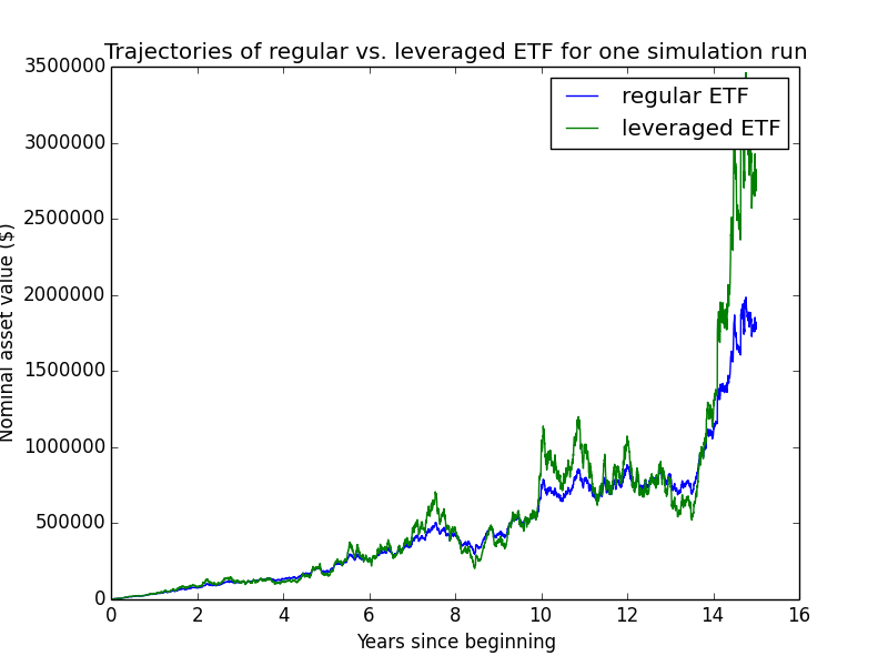
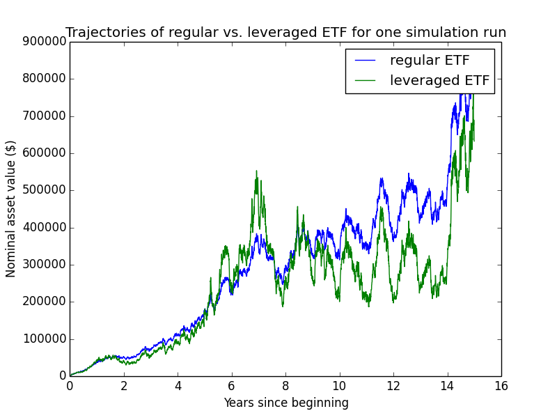
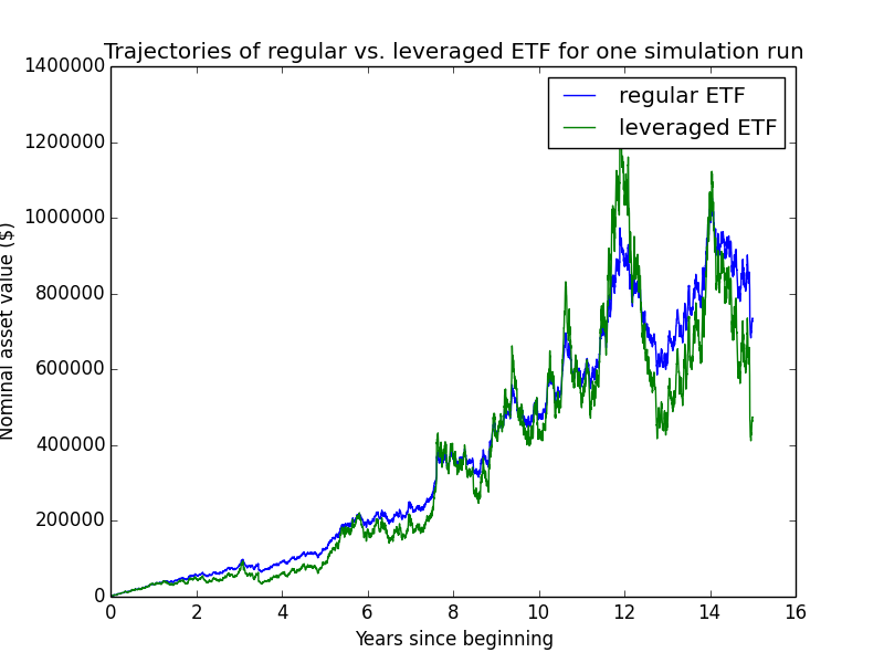
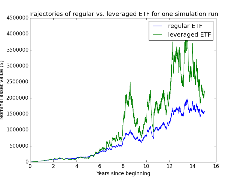
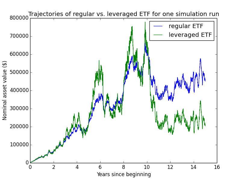
These graphs give excellent intuition for the performance of leveraged ETFs. Most of the time, even if the market goes up as a whole, the leveraged fund does worse. But every once in a while, the market goes up enough days in a row that the leveraged fund blows the regular fund out of the water. These lucky events account for a lot of the overall expected value of the leveraged fund.
Leveraged funds benefit when successive daily returns have the same sign. We can see this from the following simple calculation. Let R1 and R2 be the returns on days 1 and 2, respectively. Then the multiplier on the regular fund is
(1+R1)(1+R2) = 1 + R1 + R2 + R1R2,
while the multiplier on the leveraged fund (ignoring expenses and interest) is
(1+2R1)(1+2R2) = 1 + 2R1 + 2R2 + 4R1R2.
When R1 and R2 have the same sign, the quadratic term is positive and four times higher for the leveraged fund.
Typically the articles that warn against volatility drag from leveraged ETFs (such as this one) rig their example returns to alternate from day to day in order to make the leveraged ETF perform worse. But in practice, returns on successive days are (roughlyl) as likely to have the same sign as opposite signs.
Results vs. theory
To compare the results of my simple simulation against theory, I used basically the same leverage equations as for margin investing. The only difference is that because the expense ratio of the ETF is now significant (at least for the leveraged ETF), I include it in the equations, using the symbol f. Expenses are subtracted from a fund's NAV. So for the regular ETF:
dSt/St = (μ-f) dt + σ dWt.
And for the leveraged ETF:
dVt/Vt = (r + (μ-r)c) dt - f dt + c σ dWt.
These equations assume the expense ratio is subtracted continuously, which presumably isn't true in practice?
In order to help my simulation results match theory, I made the same adjustments as when I tried to get my margin simulation to match theory (removing inflation, black swans, unemployment, emergency savings, and salary beyond the first pay period). The following table shows the output:
| Type | Mean ± stderr | Median | Min | Max | E[√wealth] ± stderr | σln(wealth) |
| Regular | $2,421 ± $8 | $1,689 | $43 | $55,229 | 45 ± 0 | 0.85 |
| Leveraged ETF | $2,990 ± $35 | $712 | $0 | $769,599 | 38 ± 0 | 1.69 |
Leverage is better than regular 15% of the time. Leveraged account went fully bankrupt 0.0% of the time.
As you can see, leveraged ETFs usually do worse! It's no wonder they're discouraged for most investors.
Now to compare these numbers against theory:
Regular ETF
The following equations can be derived in the same ways as before. Everything is the same except that there's an extra -ft term representing the fund's expenses.
Median
empirical discounted median (from above table) = $1,689
Mean
empirical discounted mean (from above table) = $2,421 ± $8
Leveraged ETF
Median
empirical discounted median (from above table) = $712
Mean
empirical discounted mean (from above table) = $2,990 ± $35
Daily vs. monthly rebalancing
This simple leveraged-ETF simulation doesn't record actual margin or asset amounts but merely relies on the principle that the leveraged fund's daily return is roughly 2 times that of the underlying index. The approximation that the daily return is 2X the underlying return should be roughly true if the fund rebalances daily.
What if the fund rebalances monthly? In this case, the fund's return over the month isn't exactly 2X the underlying return for that month because the leverage ratio doesn't remain constant at 2X during the whole month. For instance, if the fund gained in value, its leverage would have fallen below 2X, so that the monthly return of the leveraged fund should be somewhat less than 2X that of the underlying index.
My margin simulations did keep track of margin and asset totals given daily changes in prices, and they rebalanced monthly. So if we strip away the other complexities of the margin simulation, it should approximate the simple leveraged ETF simulation but with monthly rebalancing. I presented the results for the barebones version of the margin simulation previously, but for reference, here they are again:
| Type | Mean ± stderr | Median | Min | Max | E[√wealth] ± stderr | σln(wealth) |
| Regular | $2,448 ± $85 | $1,676 | $171 | $46,213 | 45 ± 1 | 0.86 |
| Margin | $3,666 ± $594 | $847 | $10 | $550,301 | 42 ± 1 | 1.66 |
| Regular + 50% match | $3,672 ± $127 | $2,515 | $257 | $69,319 | 55 ± 1 | 0.86 |
Leverage is better than regular 21% of the time. Margin investor ended with no assets and a deficit in emergency savings 0.0% of the time. Leveraged account went fully bankrupt 0.0% of the time. Average simple-calculation margin ending balance was $3,704.
These aren't quite comparable to the daily-rebalanced leveraged-ETF results just presented because my leveraged-ETF simulations include an expense ratio, while the margin simulations didn't (or had a very tiny expense ratio in the form of trading fees). So here are the results of the leveraged-ETF simulation if the expense ratios are set to 0:
| Type | Mean ± stderr | Median | Min | Max | E[√wealth] ± stderr | σln(wealth) |
| Regular | $2,457 ± $8 | $1,714 | $44 | $56,063 | 45 ± 0 | 0.85 |
| Leveraged ETF | $3,474 ± $40 | $827 | $1 | $893,962 | 41 ± 0 | 1.69 |
Leverage is better than regular 19% of the time. Leveraged account went fully bankrupt 0.0% of the time.
With default parameters
The above results were designed to match theory. Now I show results if we use the "default" parameters from the margin simulations above, including black swans, inflation, monthly paychecks, unemployment, and emergency savings.
| Type | Mean ± stderr | Median | Min | Max | E[√wealth] ± stderr | σln(wealth) |
| Regular | $484,690 ± $1,048 | $397,571 | $47,198 | $7,403,472 | 666 ± 1 | 0.57 |
| Leveraged ETF | $531,729 ± $2,761 | $306,498 | $5,851 | $50,186,657 | 641 ± 1 | 0.90 |
Leverage is better than regular 23% of the time. Leveraged account went fully bankrupt 0.0% of the time.

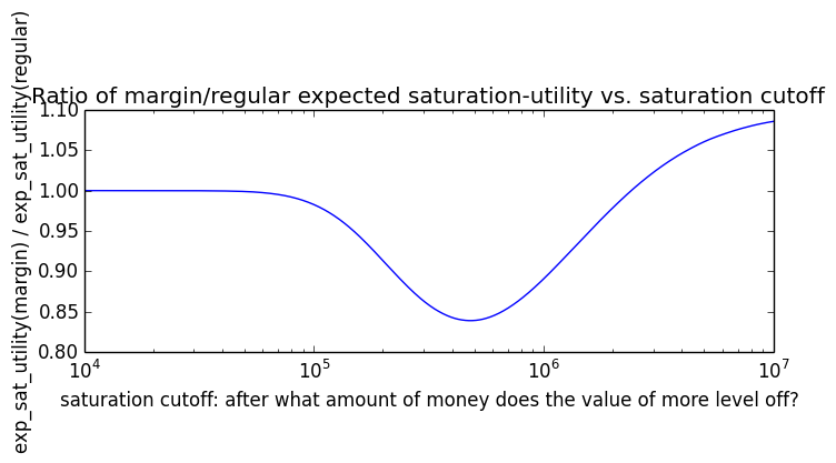
3X leverage
The following results use the same "default" parameters as above except with 3X leverage instead of 2X.
| Type | Mean ± stderr | Median | Min | Max | E[√wealth] ± stderr | σln(wealth) |
| Regular | $484,690 ± $1,048 | $397,571 | $47,198 | $7,403,472 | 666 ± 1 | 0.57 |
| Leveraged ETF | $619,278 ± $8,663 | $226,238 | $5,514 | $285,265,410 | 608 ± 2 | 1.09 |
Leverage is better than regular 16% of the time. Leveraged account went fully bankrupt 0.0% of the time.
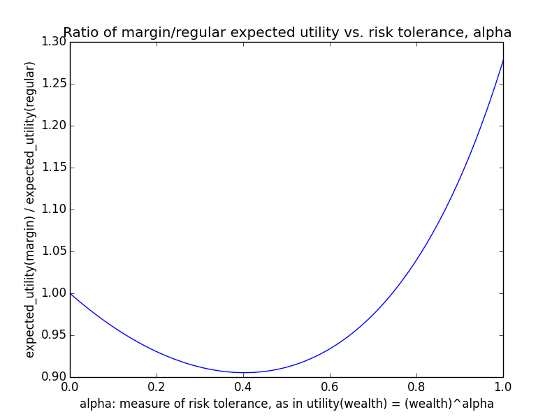
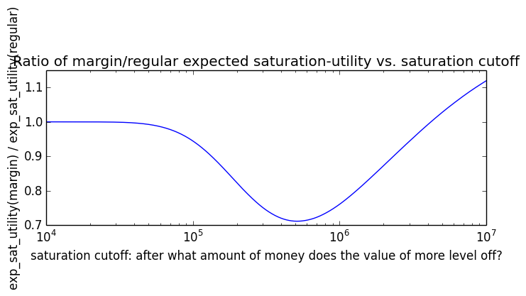
Sample trajectories:
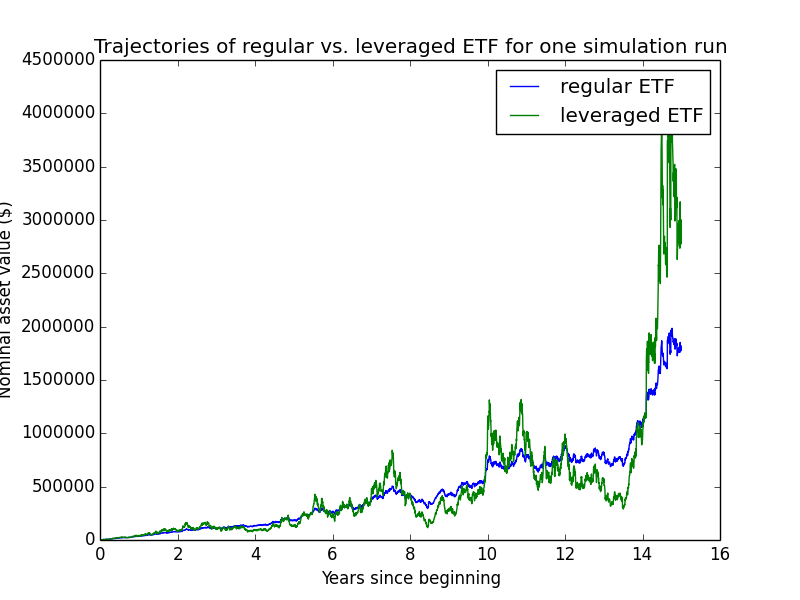
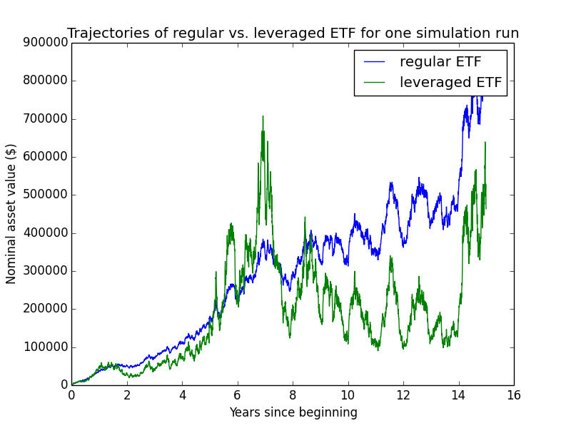
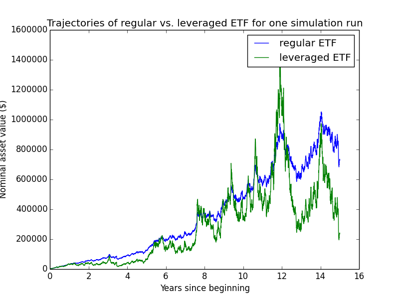
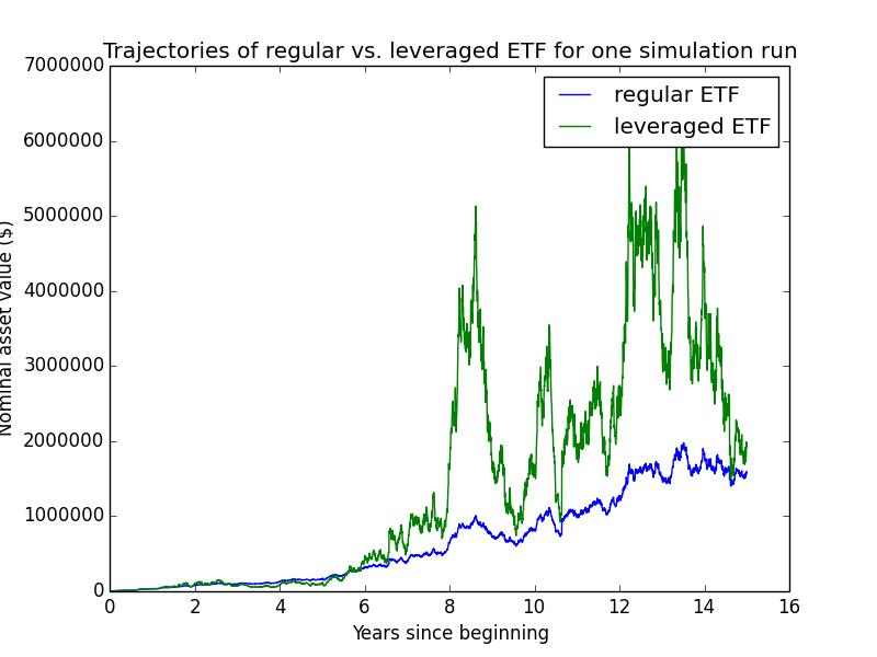
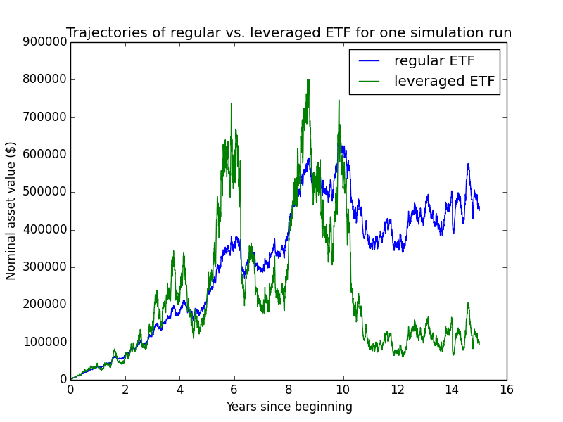
Various tax rates
As noted previously, leveraged ETFs can occasionally have unpleasant tax consequences if the fund turns over a large portion of its assets. I ran versions of my leveraged-ETF simulations that attempted to crudely incorporate taxes, by multiplying each day's return by (1 - short_term_capital_gains_tax_rate * fraction_assets_with_gains). In the "medium" tax scenario, fraction_assets_with_gains was 15%, and in the "high" tax scenario, it was 75%. (In the results presented above, the default percent of assets taxed is 0%.)
Multiplying daily returns by (1-tax_fraction) isn't perfectly accurate. If the year has a big capital loss, multiplying by (1-tax_fraction) dampens that loss as if the loss can be fully deducted. But in reality, you can't deduct more than a given amount of capital loss per year, so the (1-tax_fraction) factor may make a big loss look less bad than it would be in practice. I didn't have an easy way to fix this problem without making the simulation much more complicated. So take these results with ample sodium chloride.
Leveraged ETF only pays short-term taxes on 10% of assets per year
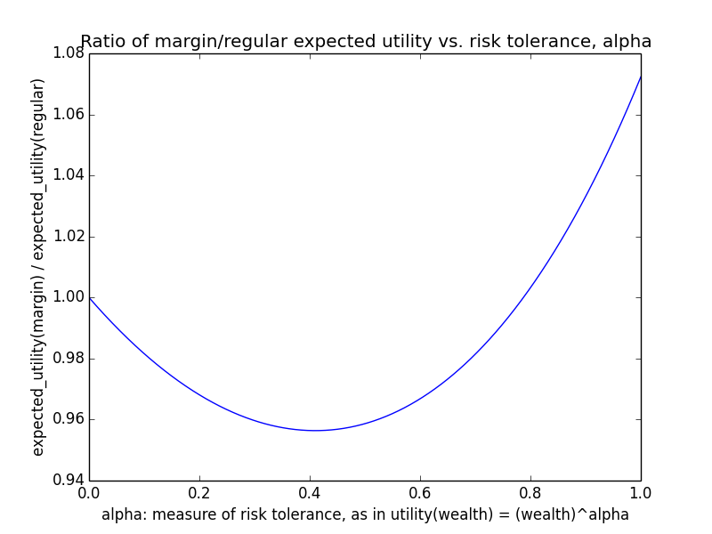

Leveraged ETF only pays short-term taxes on 50% of assets per year
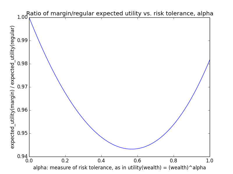
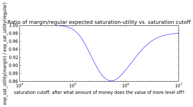
Leveraged ETFs vs. margin investing
It seems as though leveraged ETFs offer similar performance characteristics as ordinary constant-leverage margin investing. Leveraged ETFs are temptingly easy compared with do-it-yourself margin accounts.
Analysis without taxes
Apart from taxes, the main drawback of leveraged ETFs is their high expense ratios. Let's say leveraged ETFs have expense ratios of 1%, while ordinary index ETFs have expense ratios of 0.1%. Ignore the difference between daily vs. monthly rebalancing, and assume for simplicity that both forms of leveraged investing use continuous constant-leverage rebalancing. Also ignore black swans, since both approaches will face similar problems there. Say the manual work involved with managing a margin account is $W per year more than that to buy shares in a leveraged ETF. Then we have
theoretical discounted mean of LevETFt counting manual effort = LevETF0 exp{(μ-r)(c-1)t - 0.01t}
and
theoretical discounted mean of MarginAccountt counting manual effort = MarginAccount0 exp{(μ-r)(c-1)t - 0.001t} - Wt.
Assume equal starting amounts of money: LevETF0 = MarginAccountt = K. At what K does it become more cost-effective to use a manual margin account?
K exp{(μ-r)(c-1)t} exp(-0.01t) < K exp{(μ-r)(c-1)t} exp(-0.001t) - Wt
Wt < K exp{(μ-r)(c-1)t} exp(-0.001t) - K exp{(μ-r)(c-1)t} exp(-0.01t)
Wt < K exp{(μ-r)(c-1)t} [ exp(-0.001t) - exp(-0.01t) ]
Wt / ( exp{(μ-r)(c-1)t} [ exp(-0.001t) - exp(-0.01t) ] ) < K.
Suppose that managing the margin account takes 3 hours per month. On most months it would probably take far less time once you got the hang of things, but on some months you might run into problems, need technical support, etc. Also, doing taxes might be annoying.m Say your time is worth a present value of $50 donated per hour. Then W = (3 hours/month)($50/hour)(12 months/year) = $1800/year. Plugging in this and our other standard parameter values to the above inequality:
K > 1800 * 15 / ( exp{(0.054-0.03)(2.0-1) * 15} [ exp(-0.001 * 15) - exp(-0.01 * 15) ] ) = $151,420.
Here are some other values of the K threshold with different parameter inputs:
| Params different from default | Better to do manually if you invest more than ... |
| μ = .09 | $88,240 |
| W = $500 | $42,061 |
| W = $4000 | $336,489 |
| μ = .09, W = $1000 | $49,022 |
| leveraged fund's expense ratio is 0.005 | $328,356 |
| 3X leveraged fund | $105,642 |
One reason to set W high is that there's some small risk that you'll mess things up badly trying to manage the account on your own. For instance, say you have $300K invested, and there's a 1% chance that you make a mistake that costs you 10% of your assets ($30K), then this would increase W by $300 annually.
On the other hand, these numbers ignore taxes from leveraged ETFs, which might be an important additional argument favoring manual margin investing, so we incorporate taxes in the next subsection.
Finally, note that the above analysis compares expected values, but if you're risk-averse, then expected value isn't exactly what you care about. My intuition is that if you're risk-averse, the K threshold beyond which margin investing is better increases (i.e., leveraged ETFs are better for more people), because in many cases, your leveraged ETFs will decline in value, so a constant expense ratio will translate into a lower actual fee, and in the few cases where the leveraged ETF hits a home run, the fees are higher but aren't as important because the marginal value of money is lower in that case. In contrast, the cost of managing a margin account is essentially constant regardless of whether your investments perform well or poorly. Margin management costs are like a regressive tax system, which is worse for expected utility because poor people who have the least wealth value a marginal dollar more but also pay a bigger percent tax. I haven't done the math to verify that this intuition is correct or to measure how much it affects K thresholds.
Analysis with taxes
For simplicity, assume a leveraged ETF pays short-term capital-gains taxes continuously on a constant fraction F of its holdings (say, F = .05)n, with the investor's marginal short-term tax rate being R (say R = .28). Since I think ETFs carry forward capital losses, it's not too inaccurate to pretend that taxes multiply any return by (1-FR), even though in practice, an investor can't deduct losses beyond $3K/year but pays taxes on capital gains without limit.
The leveraged-ETF SDE is now
dVt/Vt = (1-FR) [ (r + (μ-r)c) dt + c σ dWt ] - f dt.
This assumes that margin interest is deductible. That's true for margin accounts. Is it also true for the implied interest that leveraged ETFs get from swaps, options, etc.?? Also note that taxes paid by the owner of an ETF aren't actually subtracted from the ETF's NAV, so this equation doesn't track the literal NAV of an ETF, just the effective NAV to a holder of the fund who pays taxes.o
Solving in the same way we solved the original leveraged Vt equation:
Vt = V0 exp{ (1-FR)(r + (μ-r)c) t - ft - (1-FR)2c2σ2t/2 + (1-FR)cσWt }.
Then, in analogy with the leveraged mean equation:
= V0 exp{ (1-FR)(r + (μ-r)c) t - ft - (1-FR)2c2σ2t/2 + (1-FR)2c2σ2t/2 }
= V0 exp{ (1-FR)(r + (μ-r)c) t - ft }.
The discounted mean is then
= V0 exp{ (1-FR)(r + (μ-r)c) t - (1-FR)μt - FRμt - ft }
= V0 exp{ (1-FR)(μ-r)(c-1)t - (FRμ + f)t }.
Modifying the ETF-vs-margin-without-taxes equation to include taxes:
Wt < K [ exp{(μ-r)(c-1)t - 0.001t} - exp{(1-FR)(μ-r)(c-1)t - (FRμ + 0.01)t} ]
K > Wt / [ exp{(μ-r)(c-1)t - 0.001t} - exp{(1-FR)(μ-r)(c-1)t - (FRμ + 0.01)t} ]
Here are some values of the threshold for various param combinations, with default F = .05 and R = .28:
| Params different from default | Better to do manually if you invest more than ... |
| default | $136,120 |
| R = .14 (this is a 28% bracket if you donate at least half your income) | $143,332 |
| F = .2 | $105,242 |
| F = .2, R = .14 | $123,812 |
Interestingly, taxes make a much smaller difference than the expense ratio. To see this, note that the expense ratio for a leveraged ETF subtracts 0.01t from the quantity in the exponent. In contrast, taxes subtract FRμt + FR(μ-r)(c-1)t = FR(μ+(μ-r)(c-1))t. Assuming low c, this is like FR * (something around .1 or .2) * t. Since F is also around .1 or .3, the result is F * (something around .01 to .06) * t. As long as F isn't close to 1 (which it's not in most years for most leveraged ETFs), taxes end up mattering less than expense ratios. Even if leveraged-ETF interest isn't tax-deductible (which means we'd ignore the -r parts of these calculations), the conclusion continues to hold. Hence, taxes may not be as much of a big bad wolf as one might have feared.
Comparison of empirical results
In order to correctly compare margin vs. leveraged ETFs, I ran a variant of margin investing where the investor tries to maintain exactly 2X leverage throughout (rather than 90% of 2X leverage as was the case in most of the results presented in this piece):
| Type | Mean ± stderr | Median | Min | Max | E[√wealth] ± stderr | σln(wealth) |
| Regular | $487,907 ± $11,052 | $395,493 | $78,803 | $4,694,052 | 667 ± 7 | 0.58 |
| Margin | $593,034 ± $33,667 | $328,822 | $0 | $22,851,993 | 670 ± 12 | 1.01 |
| Regular + 50% match | $681,900 ± $14,845 | $558,923 | $118,204 | $6,000,483 | 790 ± 8 | 0.57 |
Leverage is better than regular 31% of the time. Margin investor ended with no assets and a deficit in emergency savings 0.1% of the time. Leveraged account went fully bankrupt 0.1% of the time. Average simple-calculation margin ending balance was $583,023.
Here's a version of the leveraged-ETF simulation without expense ratios. It serves to show the differences between the margin vs. leveraged-ETF simulations (monthly vs. continuous rebalancing, taxes, etc.).
| Type | Mean ± stderr | Median | Min | Max | E[√wealth] ± stderr | σln(wealth) |
| Regular | $487,673 ± $1,055 | $399,926 | $47,403 | $7,451,677 | 668 ± 1 | 0.57 |
| Leveraged ETF | $568,034 ± $3,039 | $321,234 | $5,853 | $56,220,313 | 659 ± 1 | 0.91 |
Leverage is better than regular 27% of the time. Leveraged account went fully bankrupt 0.0% of the time.
The average ending balance of the "simple calculation" for checking the margin simulation ($583,023) is somewhat close to the average leveraged-ETF ending balance ($568,034). This is because they represent the same logical calculations. If I run each simulation for equal numbers of trials using the same initial random seed, the numbers come out identical. (TODO: Is that still true? Why are they so far apart?) I didn't run them equal numbers of times for these results because the leveraged-ETF simulations run orders of magnitude faster, so I did more iterations of them.
Now here are the leveraged-ETF results if we add in expense ratios. These are just the "Default" leveraged-ETF results from above:
| Type | Mean ± stderr | Median | Min | Max | E[√wealth] ± stderr | σln(wealth) |
| Regular | $484,690 ± $1,048 | $397,571 | $47,198 | $7,403,472 | 666 ± 1 | 0.57 |
| Leveraged ETF | $531,729 ± $2,761 | $306,498 | $5,851 | $50,186,657 | 641 ± 1 | 0.90 |
Leverage is better than regular 23% of the time. Leveraged account went fully bankrupt 0.0% of the time.
The difference between this table and the no-expense-ratios table shows the impact of the ~1% expense ratios of leveraged ETFs.
3X leveraged ETFs
Here are the same two leveraged-ETF results tables for 3X leverage to show the impact of expense ratios.
Here's without expense ratios:
| Type | Mean ± stderr | Median | Min | Max | E[√wealth] ± stderr | σln(wealth) |
| Regular | $487,673 ± $1,055 | $399,926 | $47,403 | $7,451,677 | 668 ± 1 | 0.57 |
| Leveraged ETF | $664,949 ± $9,668 | $233,343 | $5,516 | $322,407,524 | 623 ± 2 | 1.11 |
Leverage is better than regular 17% of the time. Leveraged account went fully bankrupt 0.0% of the time.
And here's with them:
| Type | Mean ± stderr | Median | Min | Max | E[√wealth] ± stderr | σln(wealth) |
| Regular | $484,690 ± $1,048 | $397,571 | $47,198 | $7,403,472 | 666 ± 1 | 0.57 |
| Leveraged ETF | $619,278 ± $8,663 | $226,238 | $5,514 | $285,265,410 | 608 ± 2 | 1.09 |
Leverage is better than regular 16% of the time. Leveraged account went fully bankrupt 0.0% of the time.
Shorting leveraged ETFs?
Because leveraged ETFs tend to decline in value, some investors short sell them, which often results in a gain. Doing this by itself seems risky, since every once in a while, the funds will perform amazingly, and then you'll lose a huge amount of money. This risk could be hedged with, e.g., long call options on the underlying ETF but at some cost to buy the options. Since a hedged position has pretty low risk, I would guess that it also has low expected return, but I haven't calculated the details.
One commenter said about a strategy of shorting both short and long leveraged ETFs: "When I wrote an article about a similar strategy back in 2009, I was contacted by hedge fund performing this. They said the biggest problem that you run into is the shares are really difficult and expensive to borrow. I don't think they are still doing the strategy anymore either."
This all seems rather complex and uncertain to me and so maybe is best left to hedge funds, though someone with more time could explore scenarios like these further.
Should you have both leveraged and unleveraged investments?
So far I've been assuming that an investor using leverage would maintain some amount of emergency funds that are invested without leverage, to fall back on if/when the leveraged investments tank. Would it be better to instead invest everything but at a lower leverage rate?
Framework
I'll focus on the case of leverage using leveraged ETFs. It can be straightforwardly extended to constant-leverage margin investing by setting the ETF expense ratio to 0 or to a low number (say, the ~0.1% expense ratio paid for typical unleveraged index ETFs).
Assume that V0 = $1, and the investor allocates some fraction θ of this initial investment toward a c-times leveraged ETF, with the rest being invested in an unleveraged ETF on the same index. (In practice, you might want to hold leveraged and unleveraged ETFs on many indexes.) For example, maybe θ = 0.5 and c = 3, in which case the investor puts half of her starting money into a 3X leveraged ETF and the other half into a normal ETF. How does this compare to putting all her money into a 2X leveraged ETF?
Let's call the final value of the mixed portfolio after t years Mt. Based on the leveraged Vt equation and regular St equation, and adding in the leveraged ETF's expense ratio f, we have
Mt = θ exp{ (r + (μ-r)c) t - ft - c2σ2t/2 + cσWt } + (1-θ) exp{ μt - σ2t/2 + σWt }. (call this the "Mt equation")
Comparing expected values
Using the regular mean equation and leveraged mean equation:
= θ exp{(r + (μ-r)c) t - ft} + (1-θ) exp(μt)
= exp(μt) [ θ exp{(μ-r)(c-1)t - ft} + (1-θ) ].
As we already would have guessed, the θ value that maximizes this is θ = 1, but investing everything in the c-times leveraged ETF is also more risky.
How does this expression compare with investing everything at an intermediate leverage amount, θc + (1-θ)? Let the t-year value of this intermediate leveraged strategy be It. Assume this leveraged ETF has the same expense ratio f as the c-times ETF does. (This seems to be a reasonable assumption in practice based on what I've seen.) Using the leveraged mean equation and adding in the expense ratio:
E[ It ] = exp{(r + (μ-r)[θc + (1-θ)]) t - ft}.
Let's simplify and look at the particular case θ = 0.5 and c = 3. Then
E[ Mt ] = exp(μt) [ exp{(μ-r)(2t) - ft} + 1 ]/2
and
= exp(rt) exp{(μ-r)(2t) - ft}.
Define U := exp{(μ-r)(2t) - ft}. Then
E[ Mt ] = exp(μt) (U + 1)/2
and
E[ It ] = exp(rt) U.
The ratio is
= exp((μ-r)t) (1 + 1/U)/2
As t approaches ∞, 1/U approaches 0, but exp((μ-r)t) also approaches ∞, which makes the ratio clearly bigger than 1. How about for smaller t? Here's the curve using μ = 0.054, r = 0.03, and f = 0.01. It starts at 1 for t = 0 and increases as t increases. So a mix of no leverage and 3X leverage has higher expected value than all 2X leverage! From this perspective, emergency savings don't optimize expected value, but they have better expected value than putting all money into a 2X fund.
Comparing expected utilities
Since most investors won't purely maximize expected value, we now examine the tradeoff for utility(wealth) = (wealth)α for some α. Analytic equations are difficult in this case, so I computed numbers empirically by drawing random samples from the relevant lognormal distributions. In particular, I sampled 10,000,000 points from the distribution of Mt given by the Mt equation and then computed expected utility for a given α. I did a parameter sweep over θ and c, checking θ values of 0, .1, .25, .5, .75, .9, and 1, paired with c values of 2 or 3, assuming a constant expense ratio regardless of leverage. The other parameters were set to their standard values as in the rest of this piece.
In the following analysis, assume that $100K was initially invested. This table shows the optimal values of θ and c, along with the expected utility for those parameters, for various values of α:
| α | optimal θ | optimal c | expected utility at optimum |
| .01 | 0.1 | 2.0 | 1.13 |
| .25 | 0.25 | 2.0 | 20.59 |
| .5 | 0.25 | 2.0 | 443.08 |
| .75 | 0.25 | 3.0 | 10110.45 |
| .9 | 1.0 | 3.0 | 81555.57 |
| .99 | 1.0 | 3.0 | 338552.74 |
It's interesting that even for α=.01, the optimal θ is more than 0. Assuming this doesn't reflect a bug in my code, this implies that even a very cautious utility function wants some balance between leverage and emergency savings.
We can also consider optimal saturation-utility for various saturation cutoffs after which money stops being valuable. Remember that the initial investment was $100K.
| saturation cutoff ($) | optimal θ | optimal c | expected utility at optimum |
| $500K | 0.1 | 2.0 | 204937.24 |
| $2 million | 0.25 | 2.0 | 232705.38 |
| $20 million | 1.0 | 3.0 | 287809.09 |
Using 3X funds to reduce expense ratio?
From what I've seen, it appears that 3X funds have roughly comparable expense ratios as 2X funds. This fact, combined with the preceding analysis, suggests that it may be better to split between unleveraged investments and a 3X leveraged ETF rather than investing more in a 2X leveraged ETF. I'm not sure if there are practical factors that militate in the other direction. For instance, could implied interest for 3X leverage be higher than for 2X leverage?
My plan for using leverage
The following was written in May 2015. It may have changed by the time you read it.
When I resume earning to give, I'll probably do something like this:
- Donate some of my earnings during the year to charities in whose value I'm already pretty confident. The main reason to give now is that the charities I want to support have only so much room to grow in a given amount of time (like a sponge has only so much room to soak up water), so it's better to donate small amounts steadily than to donate large lump sums rarely.
- If that doesn't use 50% of my income, give more to a donor-advised fund so that I've donated at least 50% of my income during that year for maximum tax deductions.
- Of remaining money not saved for retirement or spent on costs of living, invest most of it with leverage. To reduce the hassle required, I'll probably use a 3X leveraged ETF rather than a margin account. 3X leverage is ok because it's fine if I lose all of this money, since I will have already donated to the most pressing charities, and this money is just a bonus. Combining 3X leverage with an unleveraged emergency fund also might be better than just a 2X fund, though I'm uncertain on this point.
To start, I'll buy small amounts (a few hundred $) of a few leveraged ETFs. This will help me see how they're taxed and whether there are other gotchas that only become visible once you own them. I also plan to read even more literature on leveraged ETFs to make sure I'm not missing something with my analysis, given that almost everyone agrees leveraged ETFs are not suitable for buy-and-hold investors. Theory predicts that many of the leveraged ETFs I buy will lose value, so it's not as though early feedback with leveraged-ETF performance would be enough to convince me the strategy was wrong-headed.
Originally I was going to do margin investing. I might still play with it a bit to see how it goes. I've opened a margin account with Interactive Brokers. I transferred a small amount of stocks in from my previous broker so that I can play around with margin investing in a low-risk way. I also would like to go through a tax cycle before investing more in Interactive Brokers, to make sure that reporting the transactions on taxes isn't too burdensome. (Update from 2019: Tax reporting for Interactive Brokers is pretty easy. It just requires copying a few numbers from their tax statement.)
As far as retirement, the arguments in favor of contributing up to the $18K limit seem stronger to me than the arguments for investing with leverage, so I'll probably max out retirement contributions each year.
A note on refreshing this essay
I originally wrote this piece by copying and pasting static results into an HTML file. However, I kept updating my code and thus found that I had to keep refreshing the results. Eventually I parameterized the inputs and results, so that I could dynamically generate this essay from the latest run of my simulations.
That means if I find bugs, add features, or change parameters, I can rerun my program and regenerate this essay with minimal manual work. That said, generating all the results using 1000 random samples per configuration for margin investing takes 4-5 days to run on my laptop.
Footnotes
- This point is explained in a ProShares fact sheet, and you can see that the fund historically has had almost no distributions. (back)
- This equation can also be found in eqn. 10 on p. 9 of "Path-dependence of Leveraged ETF returns" with f = 0, β = c, λ = 0, and σs having a constant value σ for all s. One thing that worries me about this equation is that it depends on t. I seem to be implicitly assuming that you and all other donors have the same investment time horizon. This is obviously wrong in practice. Do my conclusions change if this assumption is ignored? I'm still very confused about this point. (back)
- If utility(wealth) is (wealth)α, marginal utility at a given level of wealth is α(wealth)α-1, which is smaller as wealth is bigger. (back)
- Buying an index fund instead of individual stocks diversifies investments. Diversification is suggested by "Understanding Investment Leverage", p. 8, item #5. That said, I would guess that buying some individual stocks would be almost as diversified, so that seems like a viable alternative to an index ETF.
While this simulation assumes you buy just one ETF on margin, you could actually buy many types of ETFs to reduce risk. Or you can assume that the ETF bought in the simulation is a global index ETF that's already fully diversified among investments, so that there aren't really further opportunities for diversification. (In practice, even if your ETF is already globally diversified, I would incline toward owning several different ETFs in case something funky happens to any particular ETF, such as if the ETF turns out to be incompetently managed or whatever.) (back)
- Tax-loss harvesting once per year is still not as good as harvesting more often. To illustrate this: Suppose you buy a security at $1000 on Jan. 1. By Feb. 1 it falls to $900. If you sell it now, you can harvest the -$100 loss. If you don't harvest now, suppose the price increases back up to $1000 by Dec. 1. Now you can't harvest the loss anymore because the loss has gone away. More frequent tax-loss harvesting does leave you with lower cost basis on your securities and hence more capital gains, but this isn't a problem if you donate the securities. Even if you don't donate them, it's better to delay capital gains because of time value of money, and long-term capital gains are taxed at a lower rate than the income from which a harvested loss can potentially be deducted. The worst that will happen is that the harvested loss will exactly offset the future capital gain that resulted from having a lower cost basis. (back)
- That said, this latter interpretation doesn't completely jive with cases where you assume that other correlated donors are also giving to the same charity, since that analysis assumed that the utility function of wealth only reflected donated wealth. If you go bankrupt, other donors aren't going to bail you out, but if you don't donate anything to the charity, other donors still will. (back)
- The cancellation isn't exact because of capital-gains taxes. In particular, suppose the market returns 5% in a year. You're deciding whether to donate $1000 now or invest it and donate $1000*1.05 = $1050 next year. If you donate now, you get a $1000 tax deduction now. Say that gets you a tax refund of $1000 * 0.28 = $280, which you invest. In contrast, if you donated $1050 next year, you'd get a $1050 * 0.28 = $294 tax refund. Even though 1.05 * $280 = $294, getting $294 one year later is slightly better because then the cost basis of your investment of the tax refund is $294 instead of $280, which means you'll pay slightly lower capital-gains taxes when you sell. (back)
- The geometric-average t-year return not compounding continuously is
Ρt := (Vt/V0)1/t - 1,
since (1+Ρt)t = Vt/V0.
Recall that in general, the continuously compounded equivalent of some return x is the number y such that (1+x) = ey, i.e., y = ln(1+x). So the continuously compounded version of Ρt is
ln(1+Ρt) = ln[ (Vt/V0)1/t ] = Rt.
- Here's the derivation. E[u(Vt)] has the form (constant) * exp( tα g(c) ), where
g(c) := r + (μ-r)c + [σ2c2/2] (α-1).
To maximize expected utility, it suffices to maximize the exponent g(c), since that's the only part of the expression that depends on c. The optimal value of c, c*, occurs where the first derivative, g'(c), is 0:
g'(c*) = 0
μ-r + σ2c* (α-1) = 0
μ-r = σ2c* (1-α)
c* = (μ-r)/[σ2 (1-α)].This is indeed a maximum of g(c) because
g''(c*) = σ2 (α-1) < 0 for α in the interval (0,1).
- In general, I use standard error for error bars because then if two error bars don't overlap, the difference is roughly statistically significant. Since the quantities in this graph are ratios (sample mean #1 divided by sample mean #2), I used a formula for propagation of uncertainty when dividing two uncertain quantities. The full formula according to Wikipedia is
if f = A/B then σf is roughly |f| √[ (σA/A)2 + (σB/B)2 - 2σAB/AB ].
For simplicity, I omitted the correlation component of the equation (the -2σAB/AB part), which only makes my error bars conservatively big given that the sample-mean margin investment performance has a high correlation with the sample-mean regular investment performance, since the sample means for both quantities will be too high when particularly good stock returns are sampled and too low when particularly bad returns are sampled. (back)
- This approach of paying off principal over time is suggested in "Understanding Investment Leverage", p. 8, item #6. (back)
- Actually, the probability of a positive daily return should be slightly higher than a negative daily return assuming the market has a positive mean return and the distribution of daily returns is symmetric about the mean, but daily volatility is so high relative to daily mean returns that the signs of successive daily returns should be basically coin flips. (back)
- Tax records for Interactive Brokers currently can't be imported to TurboTax Online, only to the desktop version with more hassle. (back)
- Note from Dec. 2017: Looking back on this article a few years later, I'm uncertain if it's correct to only focus on the fraction F of holdings that are sold in a given year. Here's an example. Suppose only half of holdings are sold each year (F = 0.5). On average, each holding would be held for two years before being sold and would thus accumulate two years' worth of capital gains before being sold. Since half of holdings would incur taxes on two years of capital gains, it's as if all holdings pay taxes on one year of capital gains. Thus, maybe I should be multiplying the return by (1-R) rather than (1-FR)? I haven't thought about this topic in a while, so maybe I'm totally wrong about this. (back)
- If you pay your ETF tax bill out of current income, then to pay $X of taxes requires more than $X of current income because that income is itself taxed. Likewise, if you paid taxes on an ETF by selling a portion of the ETF, you'd pay taxes on the capital gains from selling that portion of the ETF, so you'd actually need to sell more of the ETF so that the after-tax gain could pay off your tax bill. These considerations get complicated, but fortunately they don't affect the results that much and so can be ignored without severe loss of accuracy. Also, since I'm assuming the investor donates the ETF to charity, its capital gains are never subjected to capital-gains tax, so this equation can be read as expressing an after-tax value of the ETF (which is the same as the pre-tax value). In that case, we can interpret the tax bill as coming from after-tax dollars, in which case it's actually correct not to make further adjustments for the taxes paid on income used to pay other taxes, since all quantities in the equation are already after-tax values. (TODO: I should learn more about how ETF tax bills work to make sure this is accurate.) (back)