Summary
This page presents a calculator for the aggregate suffering of a population of an animal species based on years until the animals reproduce and how many eggs are hatched from each reproducing mother. The main selling point of this approach is that it can consider the implications of high early infant mortality rates in a more accurate way than a simple calculation could.
As expected, I find that suffering is greater when organisms have shorter lifespans because there are more deaths per unit time. Suffering also increases as organisms lay more eggs, but depending on how the population size is measured, the increase in suffering with greater egg-laying can be much less than linear.
The model used in this piece is very simplified; for instance, it assumes that mothers lay eggs only once at some constant age and that all mothers surviving to that age lay eggs. It would be good to repeat this analysis with other models to see how robust the conclusions are.
Contents
- Summary
- Epigraphs
- Motivation
- Choosing a distribution
- Simplifying assumptions about the population's dynamics
- Fitting the distribution
- Factoring in population size
- Suffering per birth
- Putting the pieces together
- Calculator for total suffering per year
- Sample suffering numbers by species
- How suffering varies with parameters
- Acknowledgments
- Footnotes
Epigraphs
Williams points out that, in all the mammalian species that have so far been carefully studied, the rate at which their members engage in the killing of conspecifics is several thousand times greater than the highest homicide rate measured in any American city.
This dark message about our furry friends is often resisted, and popular presentations of nature (in television documentaries, magazine articles, and popular books) often engage in self-censorship to avoid shocking the squeamish. Hobbes was right: life in the state of nature is nasty, brutish, and short, for virtually all nonhuman species.
--Daniel Dennett, Darwin's Dangerous Idea: Evolution and the Meaning of Life, p. 478
Many [bird] chicks don’t survive their first year: Some starve to death, their carcasses decaying [...]. Some are preyed upon by hawks or crows or cats. Some are slain by their nestmates.
We've always said [predators] kill the old and the weak. But the fact is they kill the old and the weak, and very large number[s] of the young.
--Bob Jamieson, wildlife ecologist
Motivation
When we think about the lives of wild animals, we often picture those members of a species who live to adulthood. This makes sense given that most humans live to adulthood. But for many species, most individuals die before maturity. Hence, when we're thinking about the extent of suffering in nature, in addition to counting the suffering of longer-lived individuals, we should also include the suffering of those who die young.
Ideally we'd like a mortality distribution that would show what fraction of individuals live to what ages. Then we could calculate a typical amount of suffering experienced by an individual living to a given age, and take a weighted average of those values based on what fraction of individuals live to each age.
When we get lucky, we can find life tables for a species, such as this one for a corn earworm. However, most of the time we only know more vague information, like the adult lifespan of the species and the average number of eggs laid by one mother. The piece provides a calculator that fits a mortality distribution based on lifespan and eggs-per-mother numbers in order to calculate a (very rough) estimate of aggregate suffering, counting both short-lived and long-lived individuals in a species. These numbers are obviously highly noisy, but they may at least provide rough relative comparisons among species.
Choosing a distribution
The first step is to decide on a parametric distribution for mortality, i.e., the probability density function for the ages at which individuals die. The simplest choice might be a uniform distribution, but this is pretty inaccurate for most species, where most individuals tend to die quite young. Another option is an exponential distribution. This would probably be a good fit for many species, but it doesn't work as well for some K-selected animals like humans, where mortality probability is actually higher at older ages than in youth.
For this analysis, I decided to use the Gompertz distribution, because it's standard for modeling human mortality, and under different choices of parameters, it has a similar shape as an exponential distribution. (You can see this from the top figure on the Wikipedia article for the Gompertz distribution.)
The general cumulative distribution function for the Gompertz distribution is, according to Wikipedia:
F(a; η, b) = 1 - exp(-η (eb a - 1)).
for a ≥ 0, where I've renamed Wikipedia's "x" variable as "a" to stand for "age". This function gives the fraction of starting individuals that are dead by age a. The survival function S(a; η, b) is just
S(a; η, b) := 1 - F(a; η, b) = exp(-η (eb a - 1)).
To get intuition for how the survival function S(a; η, b) behaves, here's an interactive graph of ita:
| η | b |
As you can see from playing with the graph, we can get a broad range of shapes just by varying η and keeping b fixed. (This is why η is called the "shape parameter".) For example:
- with values of η around 0.01, you can get a survival curve looking something like human mortality
- with values of η around 1 or 10 or 100, you can get an increasingly sharp exponential-type decay.b
The "scale parameter" of the distribution is b; it controls how far out the distribution goes. Smaller values of b translate to longer average lifespans.
Simplifying assumptions about the population's dynamics
For this calculator, I assume a population where births can happen at any time throughout the year, as is the case with humans and perhaps animals in tropic climates. This is definitely not true for animals in cooler climates with frozen winters, but you might be able to modify some parameters to make this calculator roughly work for those cases as well.
I assume that when people speak about the "size of the population", they're counting all individuals within the species that are at least some minimum age Amin—say, 0.05 years. (Note that all times are measured in years throughout this piece.) This helps exclude, e.g., eggs that are just hatching. If the population is aquatic and is sampled using a net with some mesh size, then the sample will tend to retrieve exactly those individuals that are above some size cutoff, which could be roughly correlated to some age cutoff.
I assume that there's an exact age Ar when females lay eggs, and they lay their whole life supply of E eggs at that time. Females who die before then lay no eggs. This assumption is untrue for many animals, but we can try to shoehorn multiple birth events into the assumption of one birth event. For example, for contemporary humans in wealthy countries, we could pretend that a female has 2.1 children (E = 2.1) at exactly 28 years of age (Ar = 28).c
I also assume that all females reaching age Ar reproduce. This is again untrue, and one extension of this calculator could be to add a parameter for the fraction of females of age Ar who actually reproduce.
I assume that eggs hatch immediately after being laid.
I ignore any potential suffering by non-hatching eggs in this analysis and only count the welfare of individuals with age after hatching greater than 0.
Fitting the distribution
Choosing η
Species where mothers leave large numbers of hatching eggs E (tens or hundreds) on average tend to be more "r-selected". These organisms typically have Type III survivorship curves. Big η values capture this shape best. η values beyond ~10 or so look fairly similar in shape, so the exact value doesn't matter that much, but higher η values become slightly more steep as far as the initial drop-off of population after individuals emerge from eggs.
η values around ~0.01 are probably more appropriate for highly "K-selected" animals like large mammals. These animals tend to have E values around, say, 2-5.d
We want a function η(E) that roughly gives us an appropriate value of η based on E. We want η(2) to be around 0.01, η(10) to be around (say) ~1, and η(100) to be some big number. (For η above like 10 or 50 or so, the shape of the survival curve remains basically constant.) One function that fits the bill is η(E) = E2/100. There's nothing special about this choice, but it's a hacky way to roughly get the kind of curve I want. That said, in the calculator, I allow you to specify any formula for η of the form x Ey + z for constants x, y, and z.
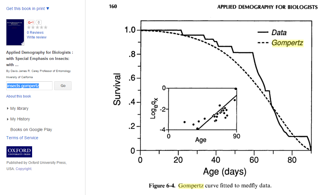
Following is an example of an actual survivorship curve fitted with a Gompertz distribution. This curve is actually more concave down than I would have expected relative to the number of offspring medflies lay (~300 per female per lifetime). I wonder if this trend is true for other insects as well.
Choosing b
In a stable population, if a mother creates E hatching eggs, on average exactly two of those hatchlings will survive to maturity and reproduce. In my framework, this means all but 2/E of the individuals have died by age Ar. That is:
exp(-η (eb Ar - 1)) = 2/E.
-η (eb Ar - 1) = ln(2/E).
η (eb Ar - 1) = ln(E/2).
eb Ar - 1 = ln(E/2) / η.
eb Ar = 1 + ln(E/2) / η.
b Ar = ln( 1 + ln(E/2) / η ).
b = ln( 1 + ln(E/2) / η ) / Ar.
Factoring in population size
Population distribution is proportional to survivorship distribution
The survivorship function S(a) tells us, given an age, what fraction of individuals born are still alive by that age. For the following discussion, I want a function N(a) that tells us, given an age, the number density of individuals currently alive who have that age. The distribution of individuals by age is sometimes called the "age structure" of the population, although often it's broken up into separate male and female graphs, whereas I intend N(a) to be the sum of males and females together.
Basically, N is a cross-sectional view of the population's age structure (one snapshot in time), while S is what one would see from a cohort study of age structure (following a given set of born individuals over time until they all die).
Let the population size be P. It turns out that in a stationary population, for all a ≥ 0, N(a) = P S(a) / (∫0∞ S(x) dx), i.e., N is the population size times a normalized version of S.
Proof:
Let S(a) be the survivorship curve as a function of age a. Let Nt(a) be the time-t distribution function of ages a in the population. That is, ∫rs Nt(a) da is the number of individuals in the population between age r and age s at time t.
Suppose a tiny increment of time da elapses. For all a ≥ 0, we have
Nt+da(a + da) = Nt(a) * S(a + da)/S(a), (call this the "N equation")
because the Nt(a) individuals that used to have age a now have age a + da, except for the fraction that died over the time interval da, and the fraction that didn't die over this time interval is the fraction surviving to age a + da, relative to the fraction that already survived to age a.
Since our population is stationary, we want to find a stationary population distribution, i.e., we want a single, t-independent function N(a) such that N(a) = Nt(a) for all t and for all a. For such a function N, the N equation requires that
N(a + da) = N(a) * S(a + da)/S(a).
Clearly one such function is N(a) = k S(a) for all a and any constant k, so k S(a) is a stationary distribution.
Since ∫rs N(a) da is the number of individuals in the population alive between ages r and s, ∫0∞ N(a) da must equal the population size, P. That means
k = P / (∫0∞ S(a) da).
In the literature on discrete Markov chains, there's a theorem about a stationary distribution being unique under certain conditions. My setup here is continuous, but assuming that a similar theorem applies, and assuming the right conditions hold (do they?), we have that k S(a) is the unique stationary distribution. ■
Counting non-measured population members
Suppose we measure the population size of a species, finding that the number of individuals at least age Amin is Pmeas. Since we didn't count individuals younger than Amin years old, the actual population size Pactual is slightly larger.
In particular,
Pactual := ∫0∞ N(a) da .
Hence:
Pactual = Pmeas * (∫0∞ N(a) da) / (∫Amin∞ N(a) da) = Pmeas (∫0∞ S(a) da) / (∫Amin∞ S(a) da).
Births per unit time
We can picture the population as is shown in the following diagram:
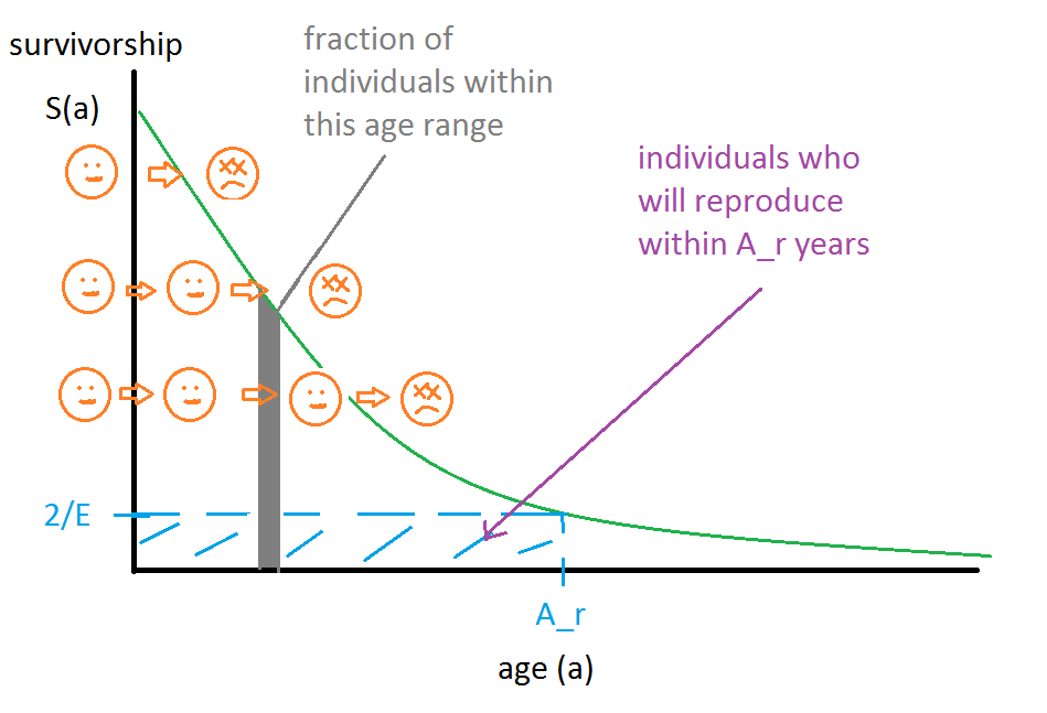
Because this is a survivorship graph, the number of individuals that die in a time interval is proportional to the difference in y values over that time interval. Since who will die at what age is deterministic, we can take a God's eye view and sort individuals along the "starting line" of the y axis such that they die at the right times. We can picture the individuals like water drops in a river that run over a curved cliff. If the stream is flowing in a stable way, then any given still-picture snapshot of the river will show the distribution of the population by survival age, which is a visual way to understand the "population distribution is proportional to survivorship distribution" theorem.
The individuals within the blue shaded region of the graph are precisely those that will reproduce within at most Ar years from now. Let the fraction of individuals in this box be R. Then the rate of individuals achieving the age of reproduction per year is R Pactual / Ar. Since each reproduction event produces E/2 hatching eggs per parent (or E hatching eggs per mother), this implies that the rate of eggs hatching per year EPY is
EPY = E R Pactual / (2 Ar).
To calculate R, we can divide the area of the blue shaded rectangle by the total area under the survivorship curve. The area of the rectangle is easy: length * width = (2/E) * Ar. The area under the whole curve is
∫0∞ S(a) da = ∫0∞ exp(-η (eb a - 1)) da.
I don't know if this is possible to integrate analytically, so for this calculator, I'm integrating it numerically.
Suffering per birth
Now that we have an expression for the number of eggs of the species that are hatched per year, all we need to calculate total suffering per year is to estimate the average suffering that results from the individual that will be born from a given egg.
Suffering given lifespan
Newborn individuals are less complex and have less developed neural wiring than adults. To quantify this effect, define a function c(a) that describes how conscious an individual is at age a, relative to how conscious it would be as a mature adult. For convenience, let's take "mature adult" to mean a = Ar. I assume that prior to maturity, c(a) has the form (a/Ar)α for some α ≥ 0. After age Ar, I assume that c(a) remains at 1. I think a good choice of α is around 1/2, which says that animals become more sentient quickly early in development and more slowly later in development. For example, if for a stone-age human, Ar = 25 (say), then a child of age 6.25 years would be considered (6.25/25)0.5 = 1/2 as sentient as an adult. (Even this seems too uncharitable toward the child, but probably for other species, especially those that develop through many distinct stages like larva to pupa to adult, this sentience curve is more reasonable.) If you want no sentience distinctions among organisms by age, you can set α = 0.
Next, we need to describe the suffering that an individual experiences with a given lifetime of Y years. For simplicity, assume that the suffering (or, if you're a classical utilitarian, you can take this parameter to be happiness minus suffering) of the individual is a constant L units per year over time (relative to its maximal consciousness at each time point). And the pain of dying (such as by predation, disease, or starvation) is a constant amount D when it happens (again, relative to maximal consciousness at that time).
So, the total suffering TS of the individual is
TS(Y) = c(Y) D + ∫0Y c(a) L da.
If Y ≤ Ar, this equals
= (Y / Ar)α D + (L / Arα) ∫0Y aα da
= (Y / Ar)α D + (L / Arα) (1/[1+α]) (Yα+1).
And if Y > Ar:
TS(Y) = D + (L / Arα) (1/[1+α]) (Arα+1) + L (Y - Ar)
TS(Y) = D + (L Ar/[1+α]) + L (Y - Ar).
Average suffering
Now that we have a function TS for the total suffering given a lifespan of Y, we need to take an expectation over the probability of having each given lifespan. We can do this using the probability density function f(a) of the Gompertz distribution, which according to Wikipedia is
f(a; η, b) = b η eb a eη exp(-η eb a).
Average suffering over all eggs is then
AS = ∫0∞ TS(a) f(a; η, b) da.
Once again, this is hopeless to evaluate analytically, so my calculator does so numerically.
Putting the pieces together
Given the above, total, population-wide suffering per year (PWSPY) is just the rate of egg production, EPY, times average suffering per egg, AS. Note that this is actually the quantity of future suffering produced by a year's worth of egg laying (i.e., the suffering those now-hatching individuals will experience over the entirety of their lives), but assuming a stable population, the amount of future suffering produced per year should equal the amount of suffering actually endured during a year. (If this weren't true, there would be either a surplus or deficit of suffering endured relative to suffering created, and since the population is stable, that surplus or deficit would be the same every year indefinitely, leading to an infinite mismatch between suffering created vs. suffering endured.)
Here's a simple example to make the point concrete. The following figure helps illustrate the text:
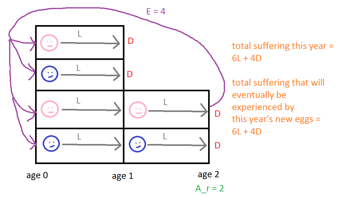
At the beginning of this year, there's a population with six individuals: four have age 0 years (two male, two female), and two have age 1 year (one male, one female). At the end of this year, two of those currently aged 0 will die, and both individuals currently aged 1 will die. Hence, total suffering this year is 6L+4D, since all six individuals live one year, and four die. (For simplicity, I'm here assuming that individuals don't become more sentient with age, i.e., that c(a) = 1 for all a.) Ar = 2, and the female individual who will reach age 2 at the end of the year will lay E = 4 hatching eggs, i.e., EPY = 4. Once laid, two of those eggs will live for 1 year, and two will live for 2 years. TS for an offspring that will live 1 year is L+D, and TS for an offspring that will live 2 years is 2L+D. AS = [(L+D) + (2L+D)]/2 = 1.5L+D. So the total suffering that will eventually be endured by the offspring laid this year is EPY * AS = 4 * (1.5L+D) = 6L+4D. This is the same as the total suffering over the current year.
Calculator for total suffering per year
PWSPY is calculated below for some default parameter values.e The units of the calculated numbers are arbitrary, but comparisons across species are meaningful. Note that if you want to compare species with different degrees of sentience, you should multiply these numbers by degrees of sentience before comparing them.
| Variable | Symbol | Value |
| Average eggs laid per reproducing mother | Elaid | |
| Hatching rate: fraction of laid eggs that hatch | hatch/laid | |
| Average eggs hatched per reproducing mother | E = Elaid * (hatch/laid) | |
| Age (in years) at which individuals lay eggs | Ar | |
| Age (in years) of individuals at which they begin getting counted in population measurements | Amin | |
| Measured population estimate (enter the order of magnitude) | Pmeas | 10^ |
| Suffering (or happiness minus suffering) per year during life | L | |
| Suffering while dying | D | |
| Exponent for sentience as a function of age relative to reproducing age | α | |
| Formula for η | η(E) = x Ey + z | * E^ + |
| Shape parameter of the Gompertz distribution | η | |
| Scale parameter of the Gompertz distribution | b | |
| Actual population (including those too young to be noticed) | Pactual | |
| Fraction of currently living individuals who will reproduce in the future | R | |
| Total eggs hatched per year | EPY | |
| Average suffering per egg hatched | AS | |
| Population-wide suffering per year | PWSPY | |
| Suffering per organism in the measured population per year | PWSPY/Pmeas |
Sample suffering numbers by species
Following are some rough comparisons among species using the calculator. The numbers are mostly driven by differences in Ar. These figures don't reflect per-species differences in brain complexity; to get the total amount of brain-complexity-weighted suffering of the species, you should multiply each of these numbers by (Pmeas of the species) * (brain complexity of the species).
| Species | Elaid | hatch/laid | Ar | Amin | PWSPY/Pmeas |
| elephantf | |||||
| mallard (Anas platyrhynchos) | g | h | i | j | |
| windowpane fish (Scophthalmus aquosus) | k | l | m | n | |
| southern green stink bug (Nezara viridula)o | |||||
| zooplankton (crustacean kinds) | p | q | r | s |
Note that if you change L from its default value of -5 to, say, +5, then the above table will show that elephants and mallards have net positive lives, but windowpanes, stink bugs, and zooplankton still have net negative lives. This illustrates the basic argument for the predominance of suffering in nature: Most wild animals have many offspring with short lives, which means that in aggregate, the painfulness of their deaths can't be outweighed even by positive lives up to the point of death.
Also, the above calculations assume that the animals reproduce year-round. If this is not the case, you can make adjustments. For example: "Nezara viridula reproduces throughout the year in tropics. In temperate zones this species presents a reproductive winter diapause [...]". So for temperate climates, if the bugs are active, say, for half the year, you could multiply the calculated PWSPY/Pmeas number by 1/2. This correction alone is not sufficient to give fully accurate results because for species where winter interrupts breeding, the population is not stationary, whereas my model assumes a stationary population. But the numbers are probably not vastly far off.
How suffering varies with parameters
Reproducing age
This chart plots suffering per organism in the measured population per year for various values of reproducing age, with all other parameters having their default values as previously set:
As expected, the amount of suffering decreases (i.e., values become less negative) with increasing lifespan.
The curve has a similar (though not identical) shape as a plot of -1/Ar. The main reason for this is the pain of death: Since death entails a given amount of pain, total pain per year from death will be (number of deaths per year)*(pain per death), and number of deaths per year is roughly related to 1/Ar (since a doubled Ar roughly translates to something like half as many eggs hatched per year, although the relationship isn't exact because the distribution of lifespans is complicated). If you set D to 0, you can see that the above graph becomes much more mild.
Eggs per reproducing mother
This chart plots suffering per organism in the measured population per year for various values of eggs per reproducing mother, with all other parameters having their default values as previously set:
You might have expected that suffering would grow almost linearly with numbers of eggs per mother because more eggs means more offspring dying young. However, recall that
EPY = R Pactual E / (2Ar).
Pactual depends on E, but it changes fairly slowly with changing E. So ignoring Pactual, we have EPY ∝ R E. The reason this isn't proportional to just E is that R is a decreasing function of E. The intuition is that if E is bigger, then more of the organisms in a given population are non-reproducing, which means the fraction of individuals who will actually become parents is smaller, and this partly offsets E being bigger.
R only partly offsets E because when the population size is measured, I assume the scientists taking the measurements count individuals that both will and will not reproduce. If we were to only count reproducing individuals as part of Pmeas, then the graph would look mostly linear. Indeed, if you set Amin = Ar, that's what you see.
Another reason the curve doesn't slope down more dramatically is that average suffering per individual, AS, is a decreasing function of E. That's because when E is bigger, organisms on average die sooner (since the survivorship curve is steeper), so the suffering of any given organism is on average smaller due to its having (1) a shorter lifespan and (2) less sentience when it dies because it's less developed.
Gompertz shape parameter (η)
If you vary the formula for η in the above calculator, you can see that the final number is extremely insensitive to it. A value of η closer to 0 (meaning that more organisms live longer lives) increases suffering per individual (since an individual's life is longer) but decreases the fraction of reproducing individuals relative to the total population size, because when a population census is taken, there are more non-reproducing animals counted (i.e., the total area under the survivorship curve is bigger).
This would be less true if we didn't count as many young, non-reproducing individuals when making population estimates. Indeed, if you set Amin closer to Ar, the final calculated numbers become more sensitive to the η formula.
Acknowledgments
One of the inspirations for this piece was some data on insect lifespans sent to me by Carl Shulman.
Footnotes
- To see the code that generates it, view the source of this page and look for the
draw()function. (back) - For values of age a near 0, if we approximate ex by 1 + x, then S(a; η, b) = exp( -η (eb a - 1) ) = exp( -η (1 + b a - 1) ) = exp(-η b a), which is the survivorship curve for an exponential distribution with rate parameter λ = η b. (back)
- Sometimes the notation mx is used to denote fecundity at a given age. However, I want E to represent the sum total of fecundity at all ages. For instance, if an animal lays 5 eggs at 2 years of age (m2 = 5) and another 4 eggs at 3 years of age (m3 = 4), E = 9 total eggs. (back)
- Yoshiaki Itō argues that the more K-selected survivorship curves are concave down rather than concave up because parental care helps reduce infant mortality. (back)
- To see the calculator code, view the source of this page and look for the
calculate()function. (back) - The top answer here suggests a female elephant can birth up to ~13 calves in a lifetime, between ages 20 and 75. Let's set Ar as the average of those ages: (20+75)/2 = 47.5. Elephants are probably counted in population estimates as soon as they're born: Amin = 0. Since elephants don't lay eggs, the "egg survivorship rate" is basically 100%, except for miscarriages.
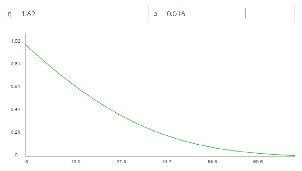
These parameter settings, combined with the other default parameter values, imply η = 1.69 and b = 0.016, giving the following survivorship curve relative to my model:
In contrast, here's an actual survivorship curve for elephants:
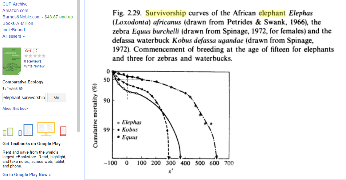
The x' variable on the x axis means "Percentage deviation from duration of pre-reproductive period" (according to pp. 50-51 of the book from which the figure comes). If I eyeball the figure around x' = 130 (roughly half of the maximum lifespan), mortality looks like it's probably ~80%, and mortality in my Gompertz-fit graph about half-way to a maximum lifespan also looks like ~80%. And if I eyeball around x' = 0 (somewhat less than 1/4 of the maximum lifespan), mortality looks to be around ~65%? And on my Gompertz-fit graph, mortality a bit less than 1/4 of the way to the end looks to be about ~40%. So my Gompertz fit is good but not perfect. (back)
- This page reports a clutch size of 11 - 14 eggs (average = 12.5). Assuming a mother lays only one clutch (how true is that?), this gives Elaid = 12.5. (back)
- This book reports (p. 70, Table 2.7) that 49% of eggs hatch for US mallards. (back)
- This page says mallards begin breeding at 1 year old and have a typical lifespan of 3 years conditional on having reached breeding age. The average number of breeding years conditional on reaching breeding age is thus 3 - 1 = 2, and the average age at which the birds would lay eggs would be (2 average breeding years) + (1 year to start breeding) = 3. (back)
- I'm just making this up. (back)
- I didn't find numbers for this specific species, so I'll make guesses based on other fish.
This source reports an average of 11,141 eggs per mother salmon.
This book reports 4500 eggs laid on average for sockeye salmon, with a 99.97% mortality rate between eggs and adult fish. The book also presents the following information on eggs laid per mother for several fish species:
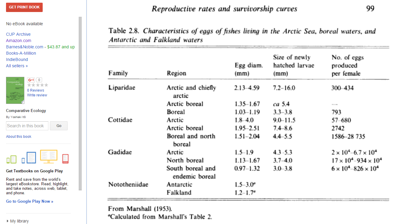
This book chapter reports numbers of eggs laid per pound of fish that are mostly in the hundreds, thousands, or tens of thousands. Given that a windowpane fish "Seldom exceeds weights of 350 to 400 g", it weighs a bit less than a pound.
My overall point estimate for this parameter is 5000, which seems somewhere in the middle among these numbers.
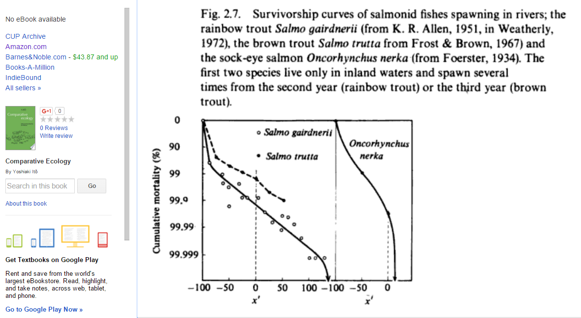
By the way, here are some actual survivorship curves for fish (from p. 55 of this book):
 (back)
 - I didn't find numbers for this specific species, so I'll make guesses based on other fish.
This study found that 39.68% of Clarias gariepinus fish hatched in the "control" condition.
Another study found that an average of 90.3% of rainbow trout eggs hatched in the "control" condition (Table 2, p. 147). The study notes (p. 148) that this number is comparable "with survivals of 90 to 95% for the hatchery program from which the fish were obtained (M. Albert, personal communication, 1976), as well as with published values for other studies using rainbow trout (Anon. 1973)".
I'm not sure if these numbers for percent of eggs hatching are higher than would be the case in the wild. But for now I'll assume they're roughly accurate and take a point estimate of 50%. (back)
- This document reports that "Sexual maturity occurs at 3-4 years of age [...] (O’Brien et al. 1993)." (back)
- This document reports that "Fish spawned in the spring grow quickly and reach sizes of 11-19 cm TL [total length(?)] by September, about four months after spawning. By the following spring, most fish of this cohort are larger than 16 cm TL. Fish spawned in the autumn are 4-7 cm TL in December and reach 18-21 cm TL by the following October (Morse and Able 1995; Able and Fahay 1998). [...] Windowpane attain a maximum total length of about 46 cm (Scott and Scott 1988)." So let's say it takes ~3 months (just making this up) before the fish become big enough to be counted in population estimates. (back)
- Below is a figure from this book (p. 84):
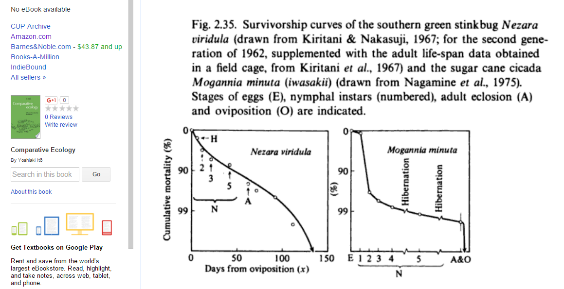
It's one of many survivorship curves for insects presented in that book, but I'll focus on Nezara viridula. I think this survivorship curve shows egg mortality as part of the curve. Mortality before reproduction is around, say, ~92% (give or take), i.e., 2/Elaid = 0.08 so that Elaid = 25.We can also read off an approximate hatching rate from the graph, since I think the "H" denotes "hatching". H is about 1/5 of the way down to 90%, but the y-axis scale is logarithmic, i.e., if p is the cumulative mortality between 0 and 1, then the y distance down from the top is proportional to y(p) = log10(1/[1-p]). (To see this, note that for p = 0.99, y(p) = 2, while for p = 0.9, y = 1.) So we want the p such that y(p) = 1/5:
log10(1/[1-p]) = 0.2
1/(1-p) = 1.58
1-p = 0.63
p = 0.37.This jibes with estimates of egg mortality for other insect species:
- In this life table for a corn earworm, out of 1000 eggs, 382 made it to the first larval stage, suggesting a hatching rate around 0.38.
- This book reports findings by Zhou et al. (2009) that H. oblita hatched at rates between 2.1% and 75.6% depending on soil moisture.
Time to maturity for Nezara viridula in the above figure looks to be around ~65 days, i.e., Ar = 65/365 = 0.18. I'll just randomly guess that Amin might be, say, around the time of the second instar of that species, which from the graph looks like ~10 days = 0.03 years.
These parameters imply η = 0.86 and b = 5.7, which has the following fitted Gompertz curve:
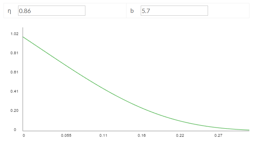
If you eyeball this fitted curve against the empirical Nezara viridula curve, it looks like it doesn't fit that well, but part of the reason is that the empirical curve starts from egg laying as age a = 0 and S(a) = 1, whereas my fitted curve starts from egg hatching as a = 0. Once you account for ~37% egg mortality, the fitted curve corresponds with the empirical curve reasonably well, though far from perfectly. (back) - This page reports that "females [...] produce 10 to 40 eggs per clutch [...] (Balcer et al., 1984)". This book notes: "most crustacean zooplankton produce only a few hundred eggs per female (see Paffenhöfer and Harris, 1979, for review)". I took 100 as a round number to serve as my point estimate. (back)
- This study reported "Mortality of hatchlings [of] (68 vs. 69%)" for zooplankton, although the authors think these numbers might have been high: "The observed high mortality rates may be due to the limitations of the small static cultures or to the fact that only one species of algae was used as additional food source."
A second study found hatching rates of ~1/2 to ~3/4.
A third study found relatively high "hatching success" rates within 15 days (around ~60% to ~100%—see Fig. 2, p. 1977) but noted that past studies had found pretty high apparent egg mortality rates in the wild—typically in the range of 30-99% per day (Table 1, p. 1972). The study concludes (p. 1985) that one reason for the higher apparent mortality in the wild may be that, in the wild, eggs sink to bottom sediments before hatching.
A fourth study found hatching rates of ~40% to ~100% after 35 hours depending on temperature.
Overall, the estimates are variable, but I chose a 50% mortality rate as a round number somewhere in the middle of the above data points. (back)
- This page reports that eggs "take from 28 to 35 days to develop (Balcer et al., 1984)". There's additional latency between when eggs are laid vs. when they hatch, but in the majority of sources I looked at, this was small (on the order of 5-10 days), and since my model ignores this latency, I'll ignore it here. So let's say 31.5 days to develop: Ar = 31.5/365 = 0.086. (back)
- I'm just making this up. (back)